
Predicting Income from Census Data
The goal of this data science project is to predict if an individual makes greater than or less than $50K based on certain attributes using R. The data set is sourced from the 1994 United States census and is provided by the UC Irvine Machine Learning Repository. I fit my model using a logistic regression to better understand the effect of various variables on the likelihood that an individual earns more or less than fifty thousand dollars. You can find my source code on Github.
About the Data
The data set is composed of two partitions: training and test data. The data was split using MLC++ GenCVFiles with ⅔ of the data serving as training data and ⅓ serving as testing data. The training data set is composed of 32,561 observations and the test data is composed of 16,281 observations. The data set includes 15 variables: 6 continuous and 9 discrete.
Continuous Variables
age
fnlwgt
education-num
capital-gain
capital-loss
hours-per-week
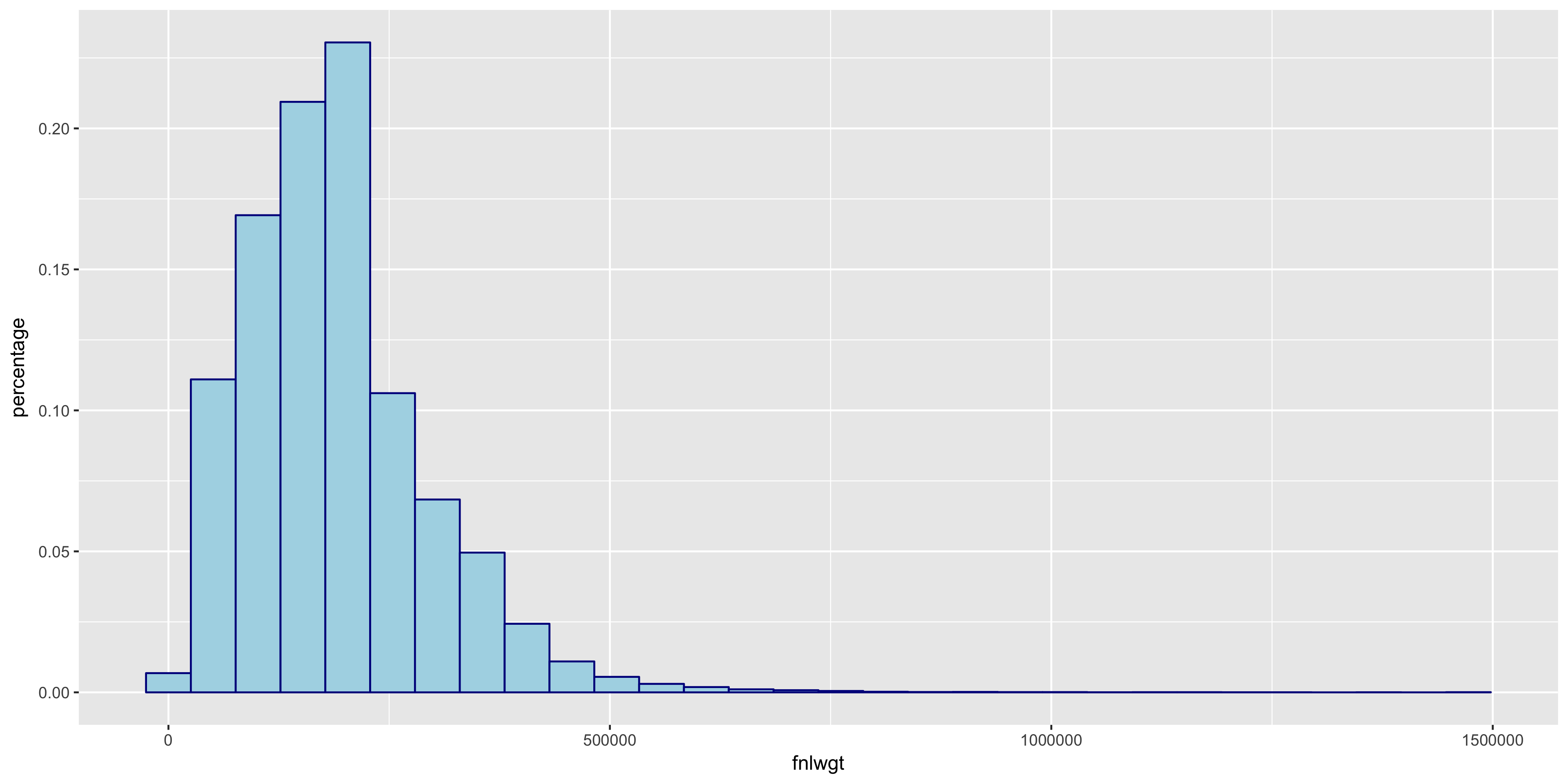
Description of fnlwgt
fnlwgt is the final sampling weight. This measure is included because a portion of the United States population is unable to complete a census including citizens in incarceration and active duty military members. The inclusion of final weight attempts to correct the systematic differences in selection probabilities.
Discrete Variables
>50K or ≤50K
workclass
education
marital-status
occupation
relationship
race
sex
native-country
The target variable is the >50K or ≤50K discrete variable.
There is a possibility of unknown values in the data set and they are represented by ‘?’s in the data. 3,620 observations include unknown values.
Exploratory Data Analysis
Before we jump right in to creating a classification model, let’s first learn about our data.
Explore Continuous Variables
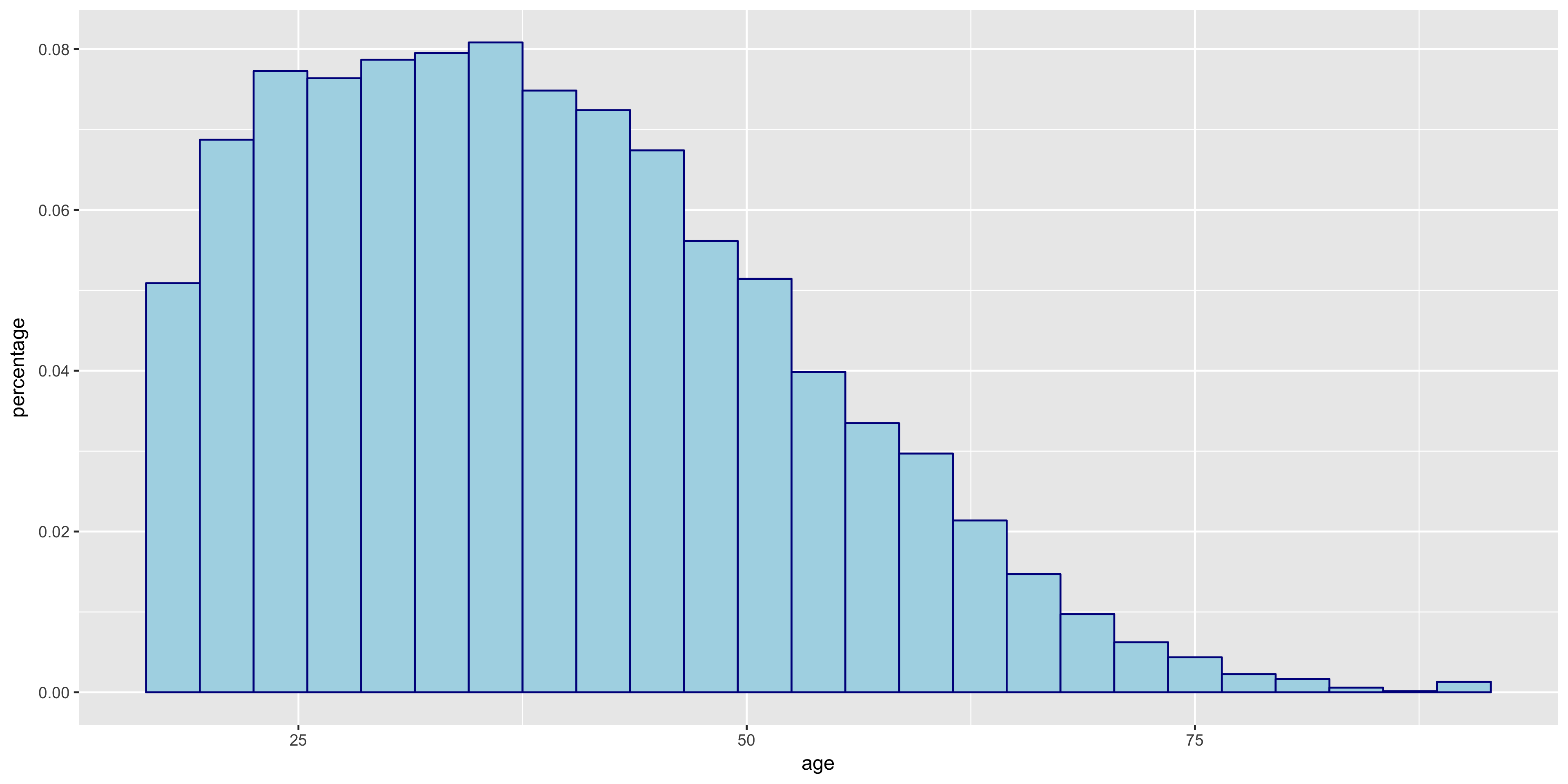
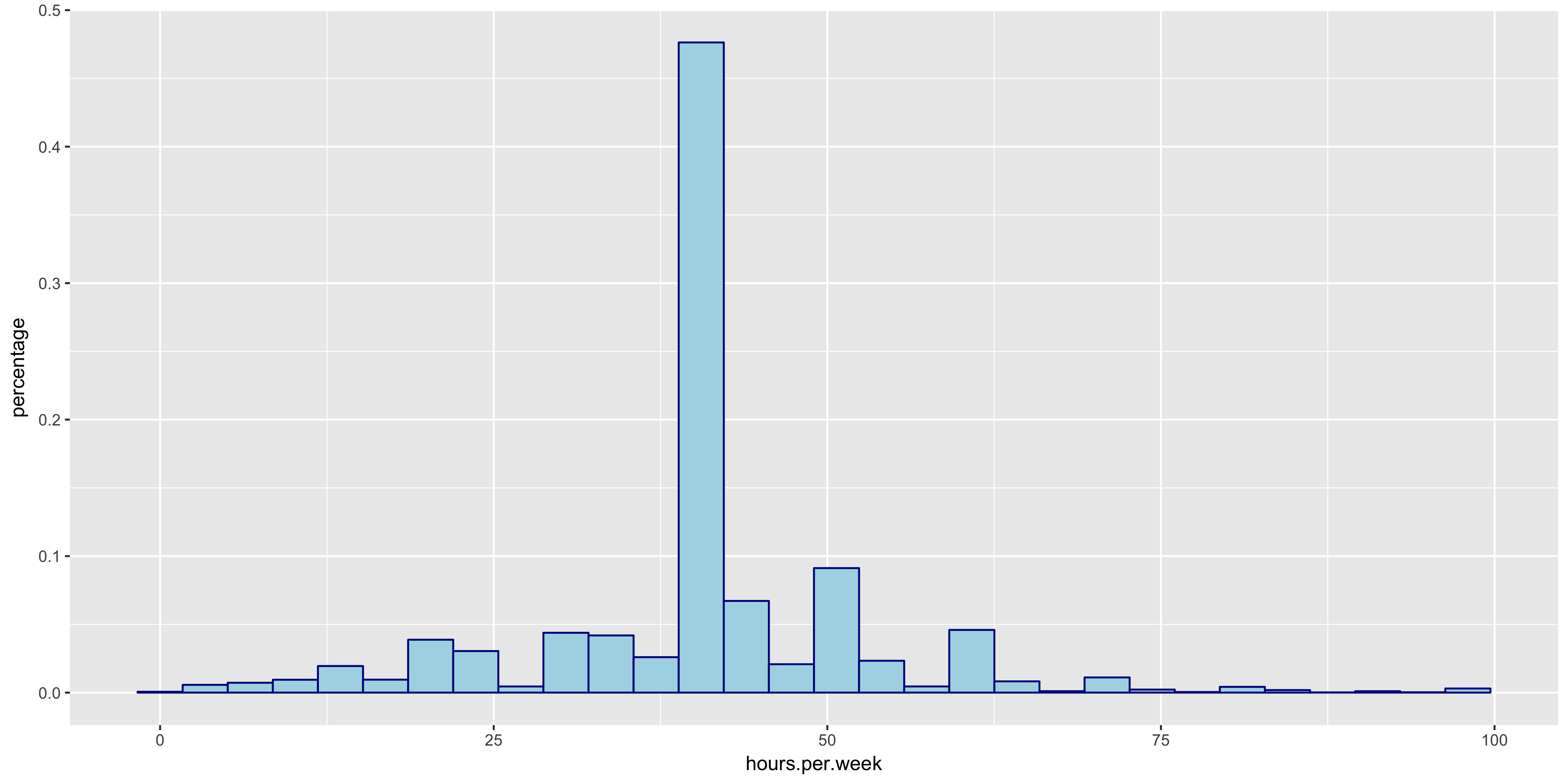
I began my exploratory data analysis by first examining the continuous variables. I created relative frequency histograms for each variable using the R libraries ggplot2 and gridExtra.
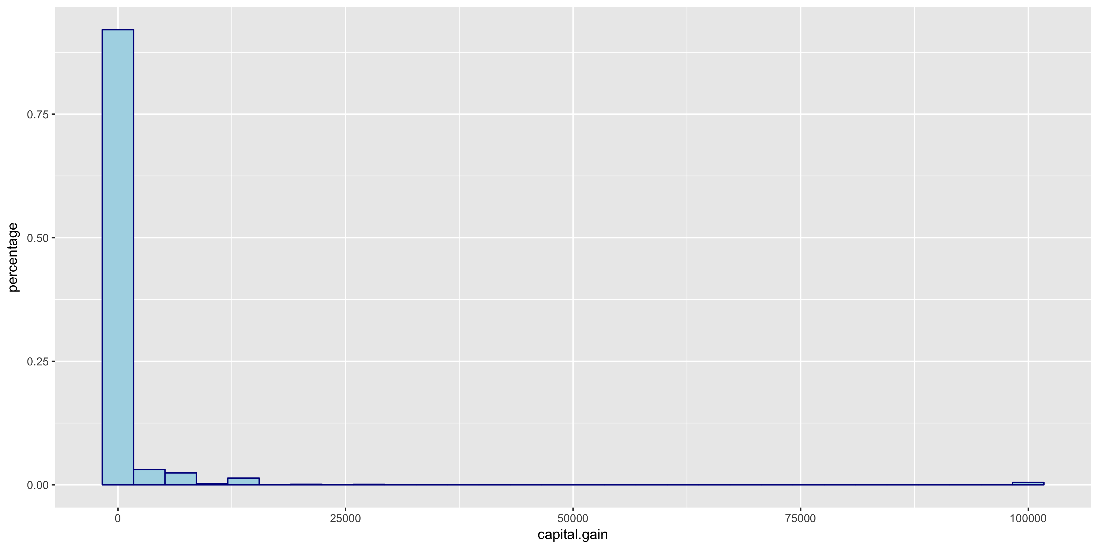
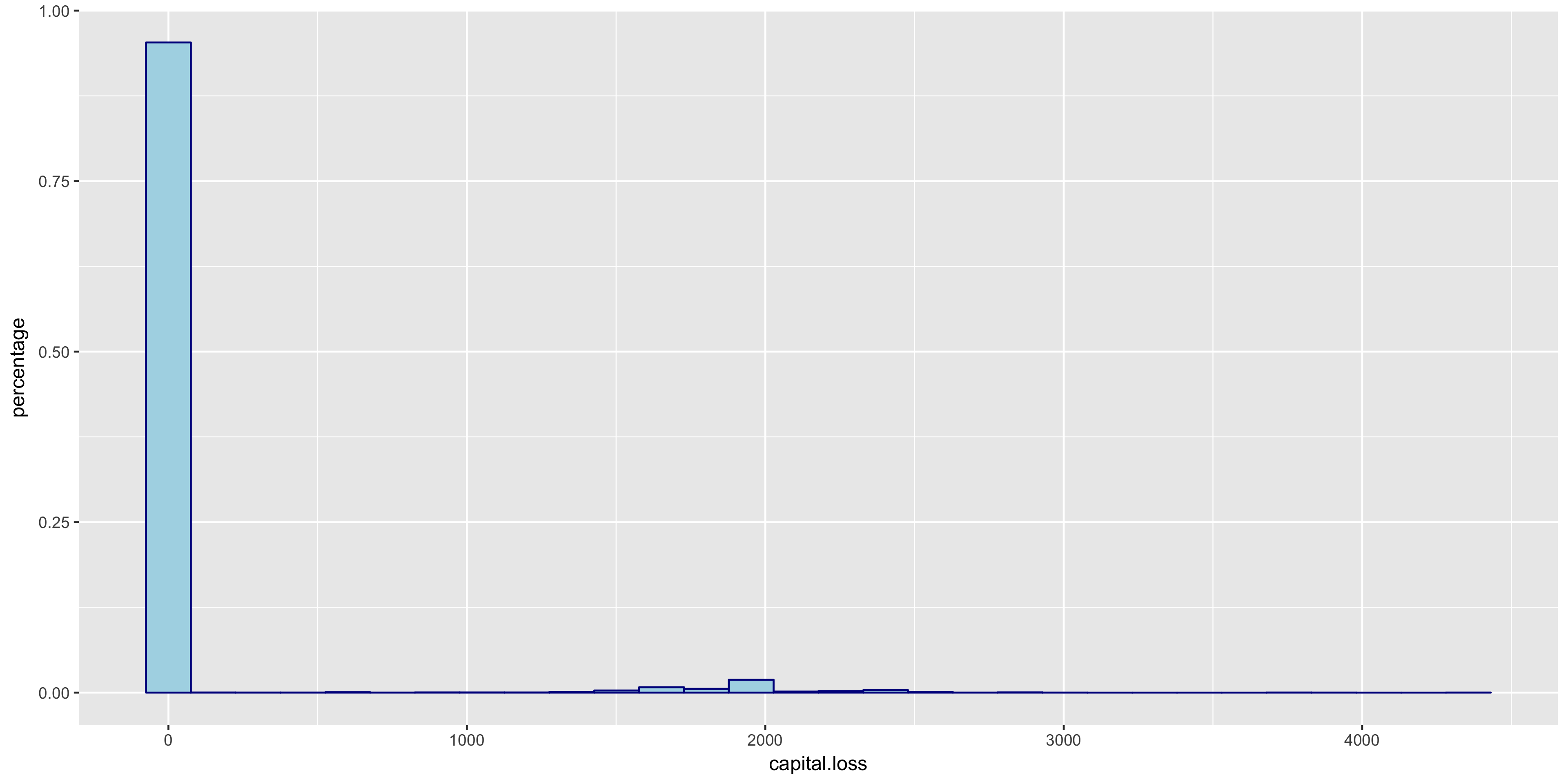
The relative frequency histograms of capital gain and capital loss lead to valuable insight. Since both of the variables are very tightly distributed at 0, I will not include them in my initial model.
To further explore the continuous variables, I created box plots of the remaining variables to compare the above 50K and below 50K distributions.
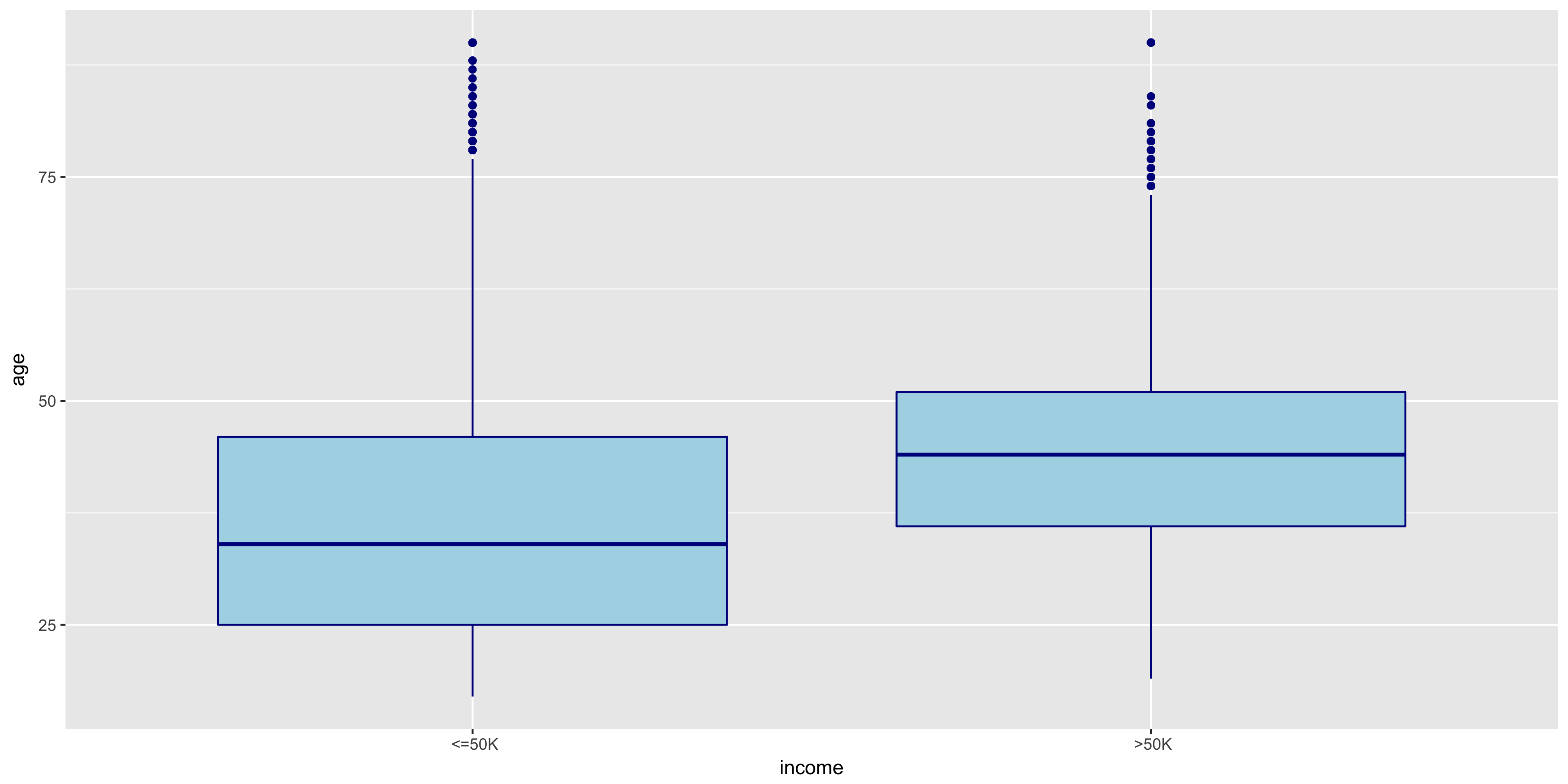
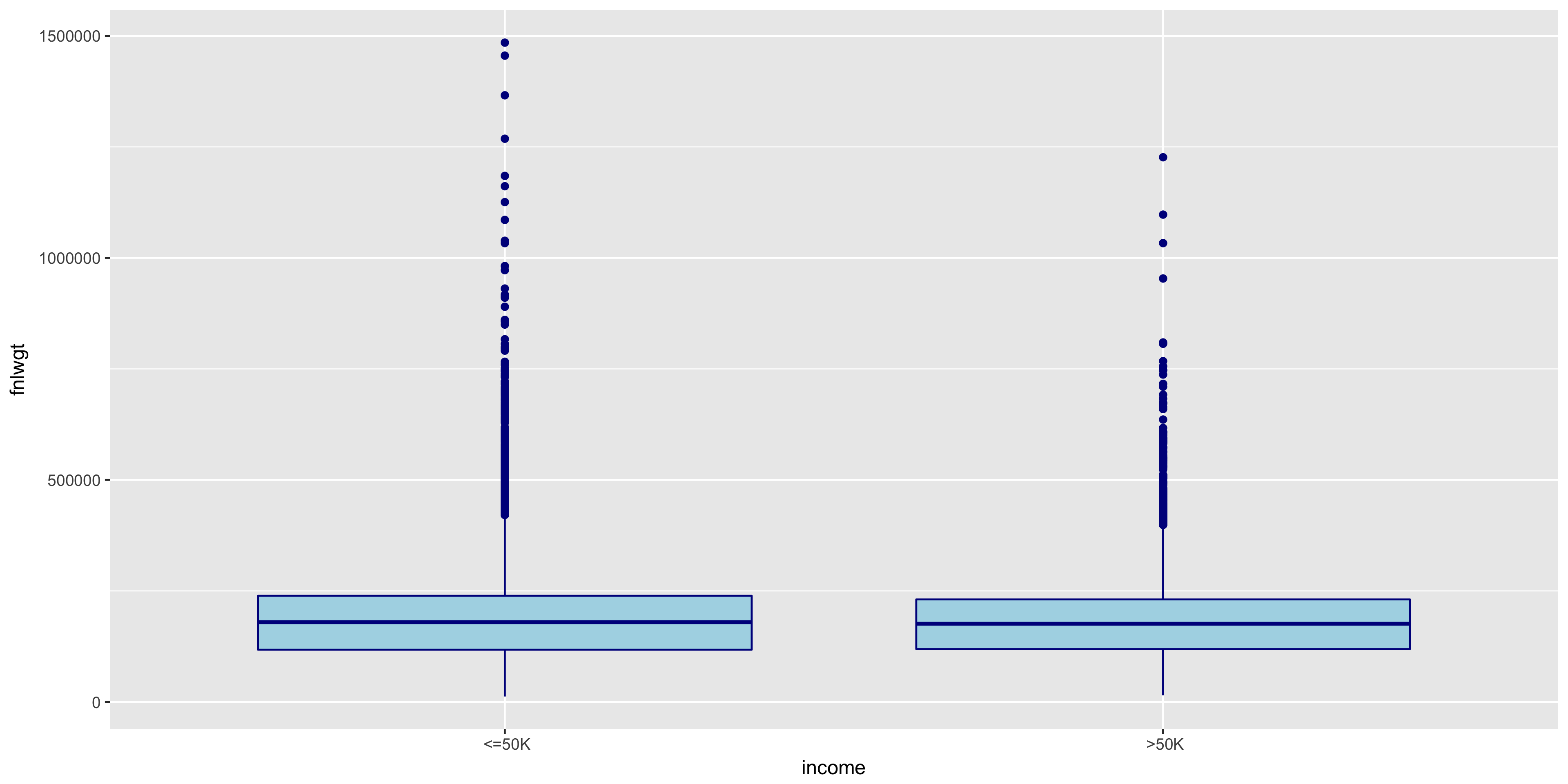
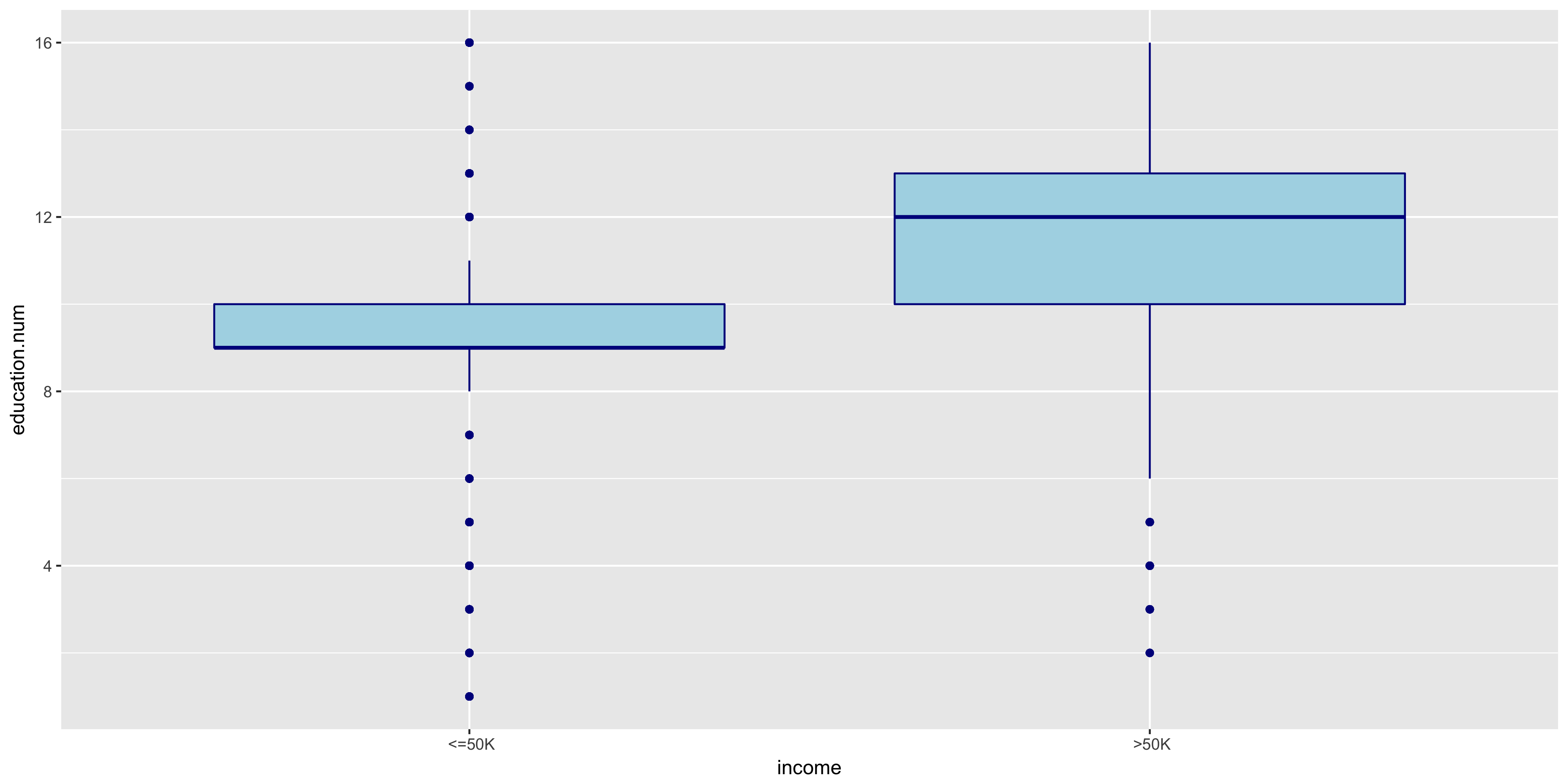
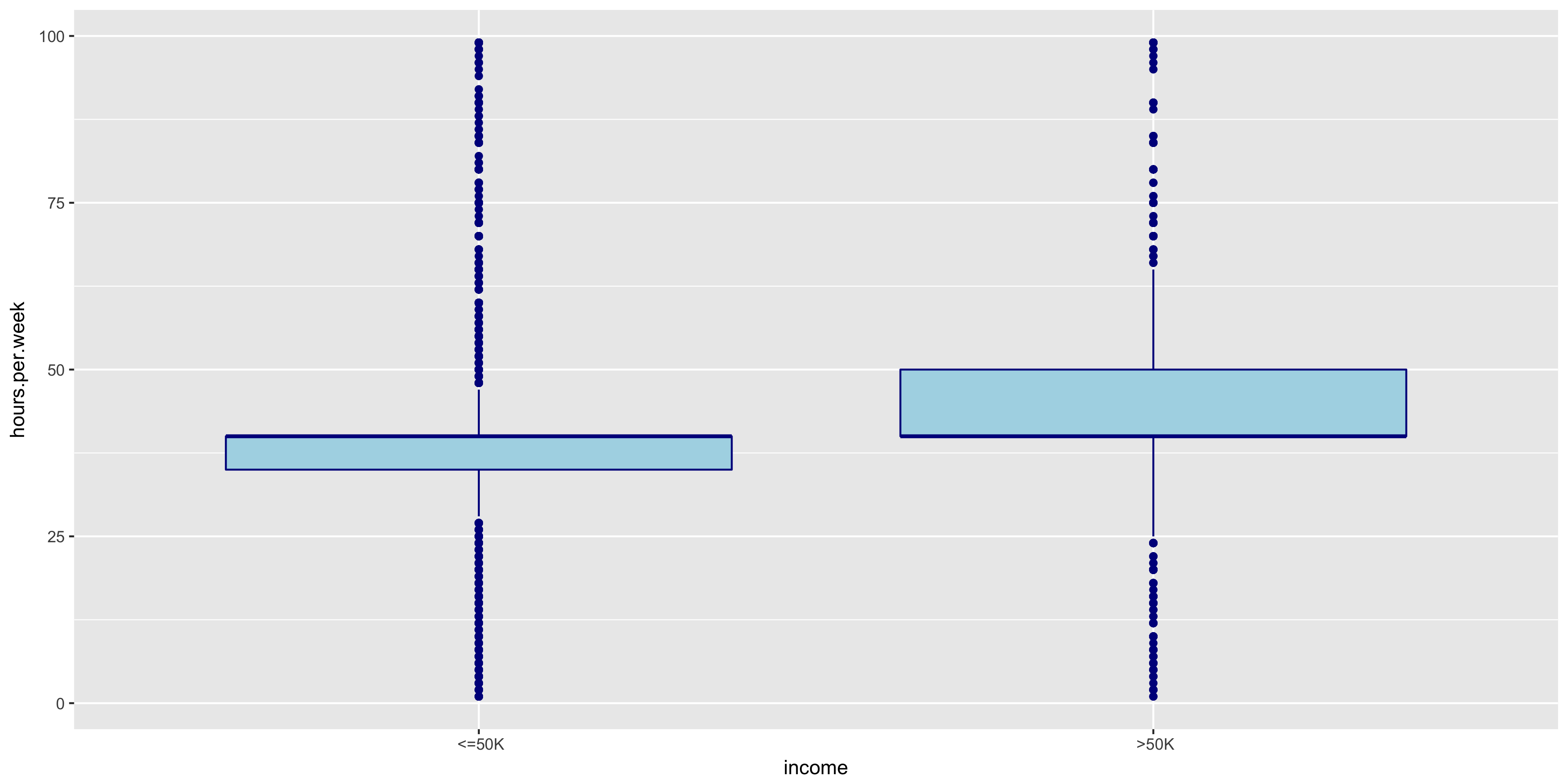
The distributions of >50K and ≤50K in the fnlwgt box plot are nearly identical. For this reason, I will not include fnlwgt in my initial model. The >50K distribution seems to correlate to higher education levels.
Explore Discrete Variables
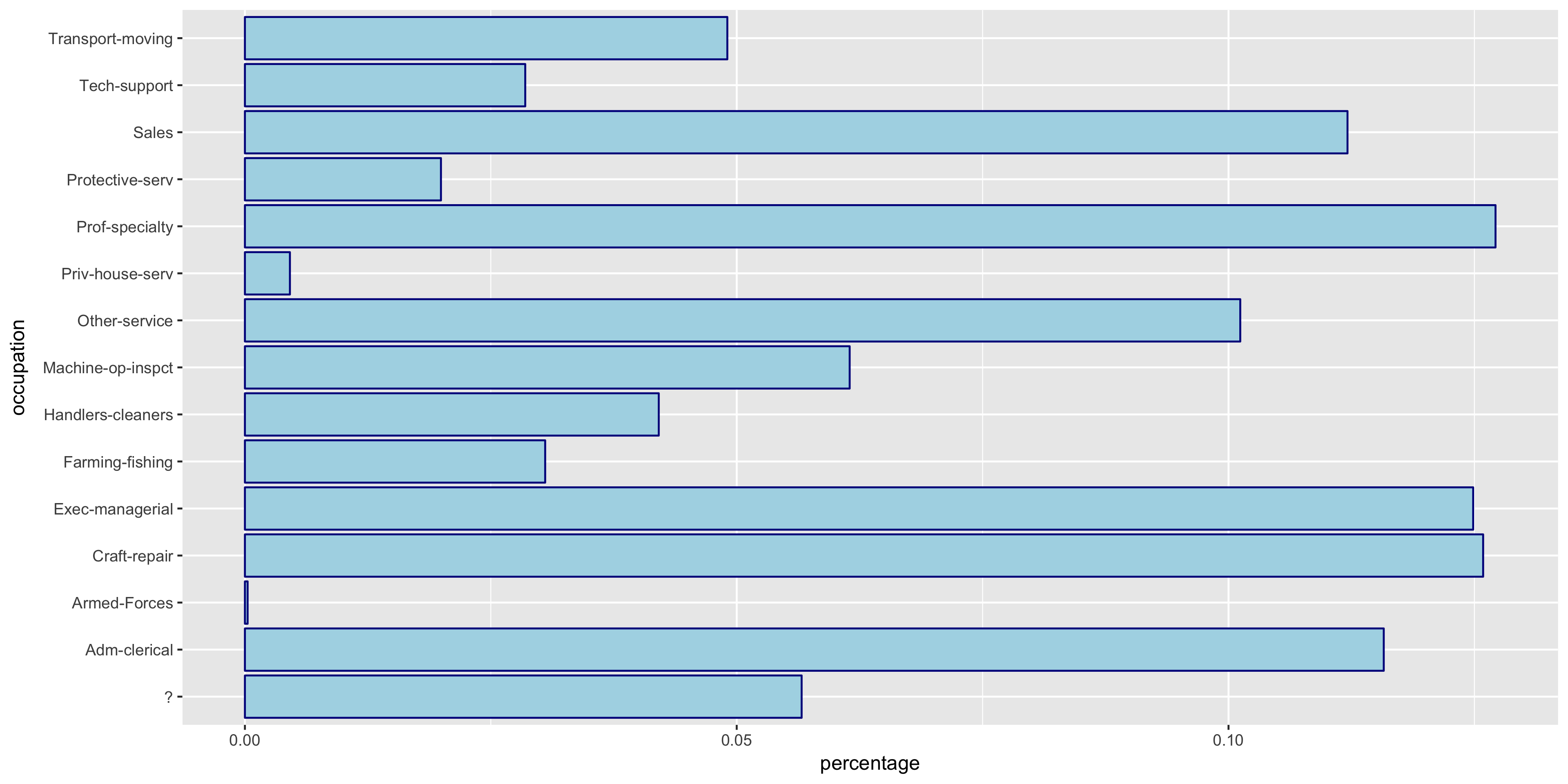
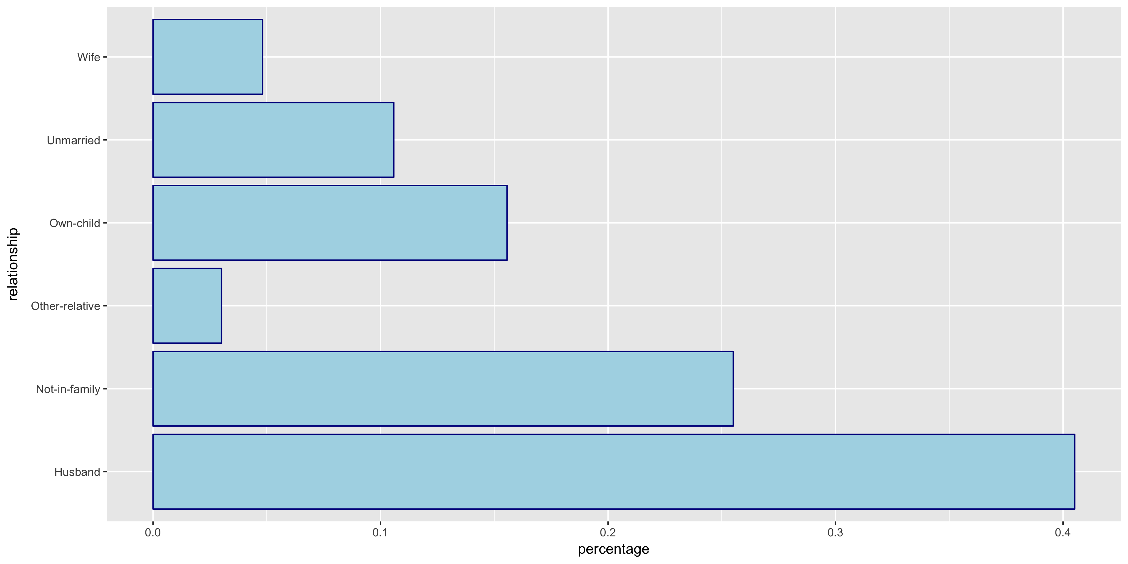
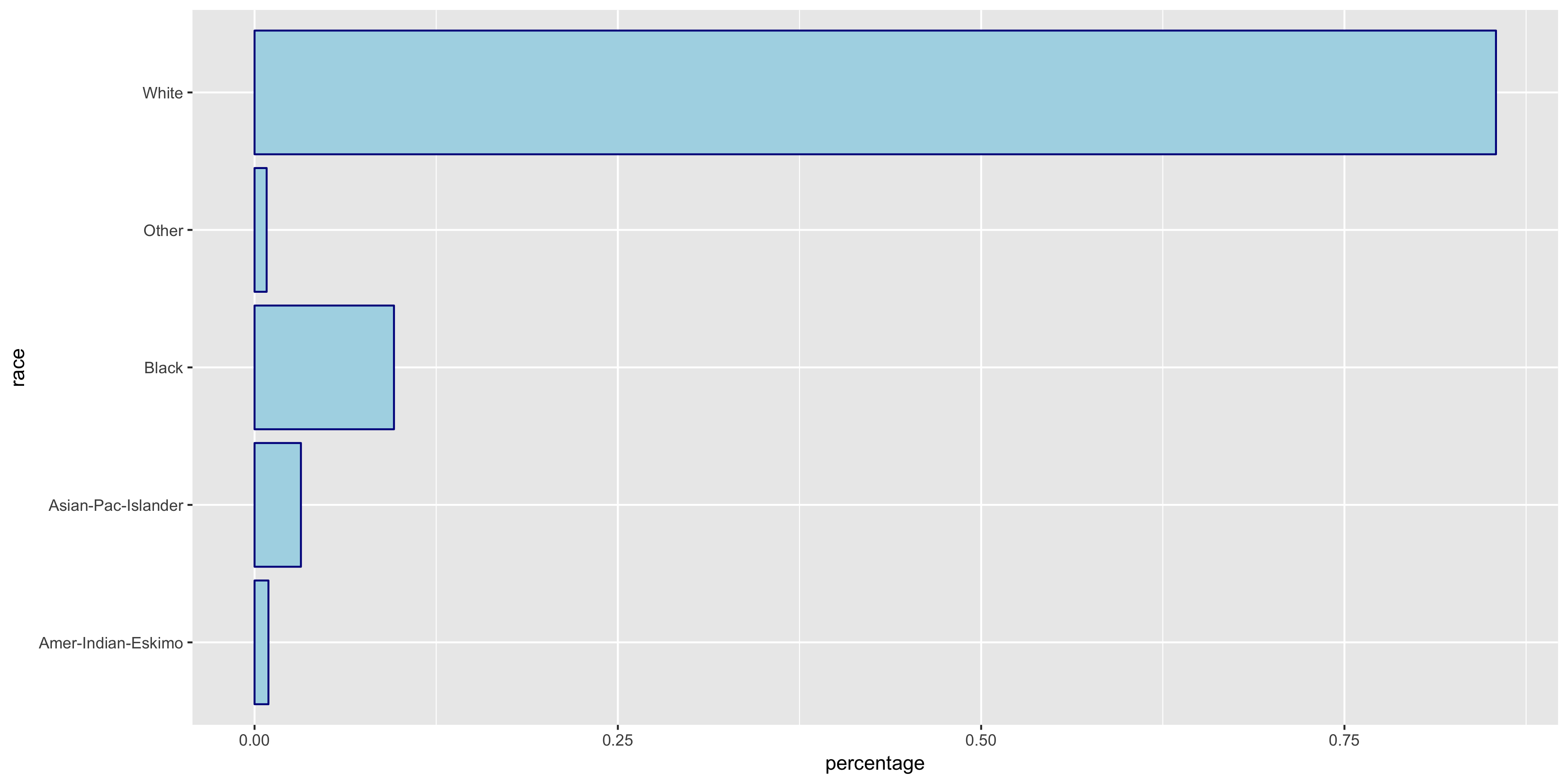
To begin my exploratory data analysis on the discrete variables, I plotted the relative frequency bar graphs as opposed to the histograms for the continuous variables.
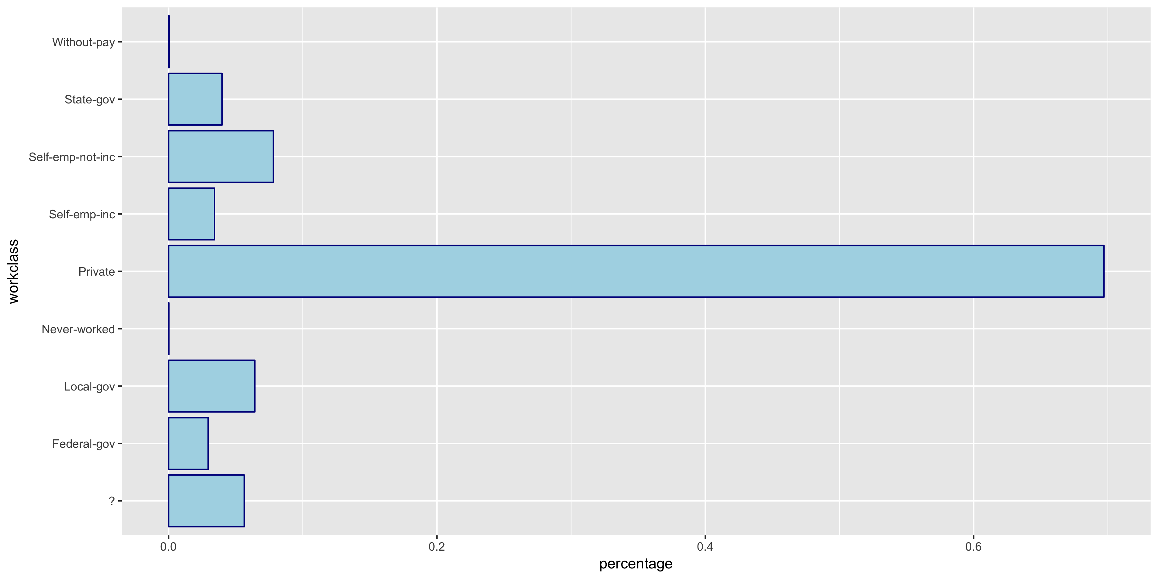
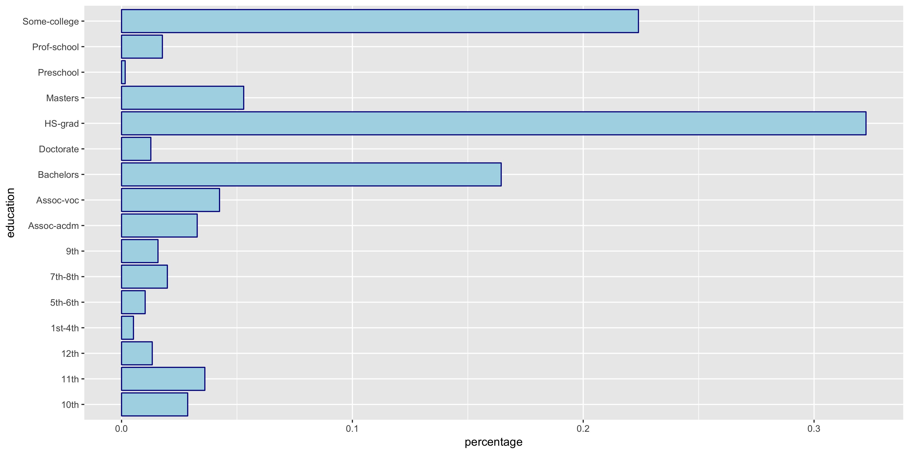
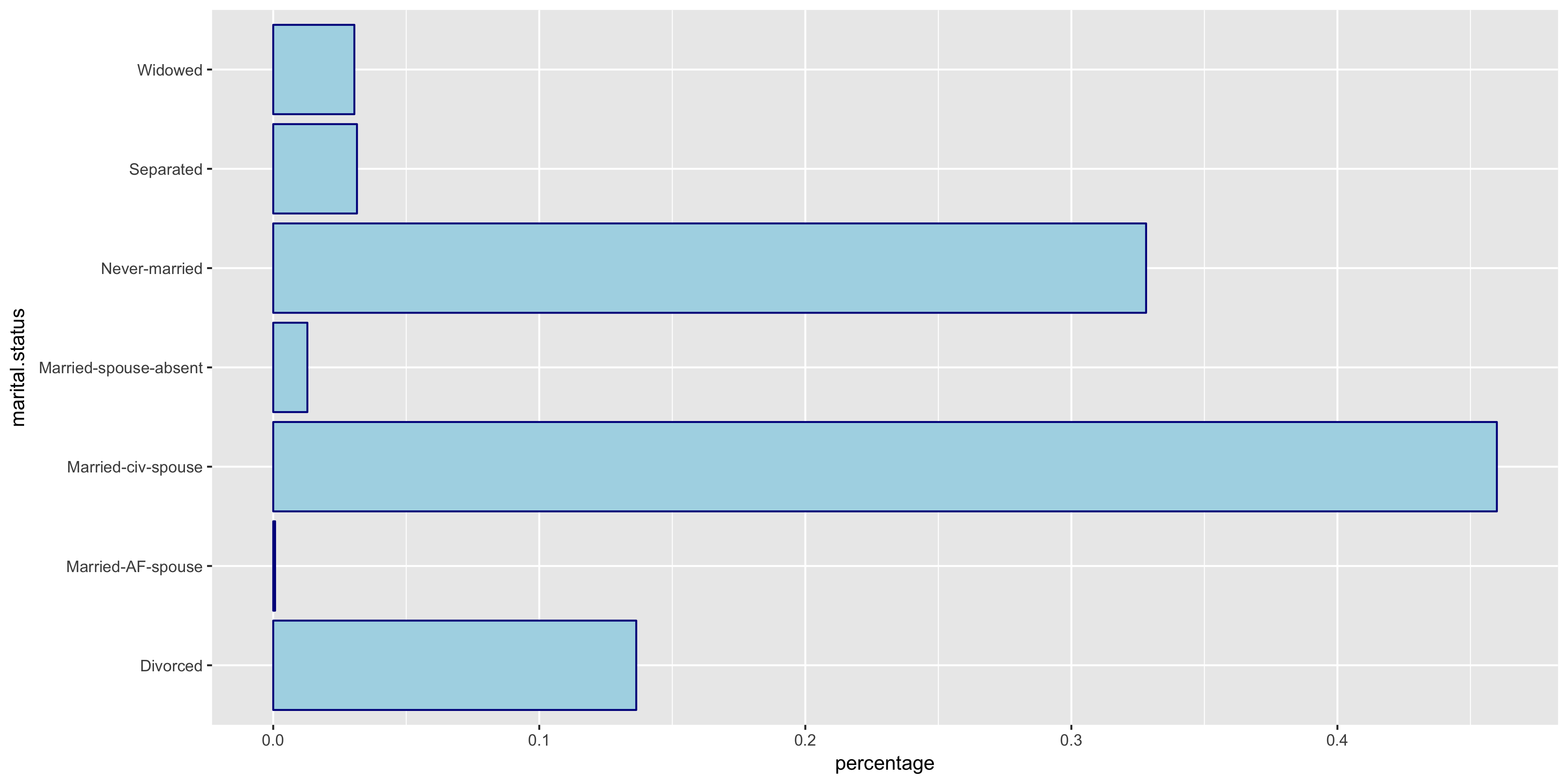
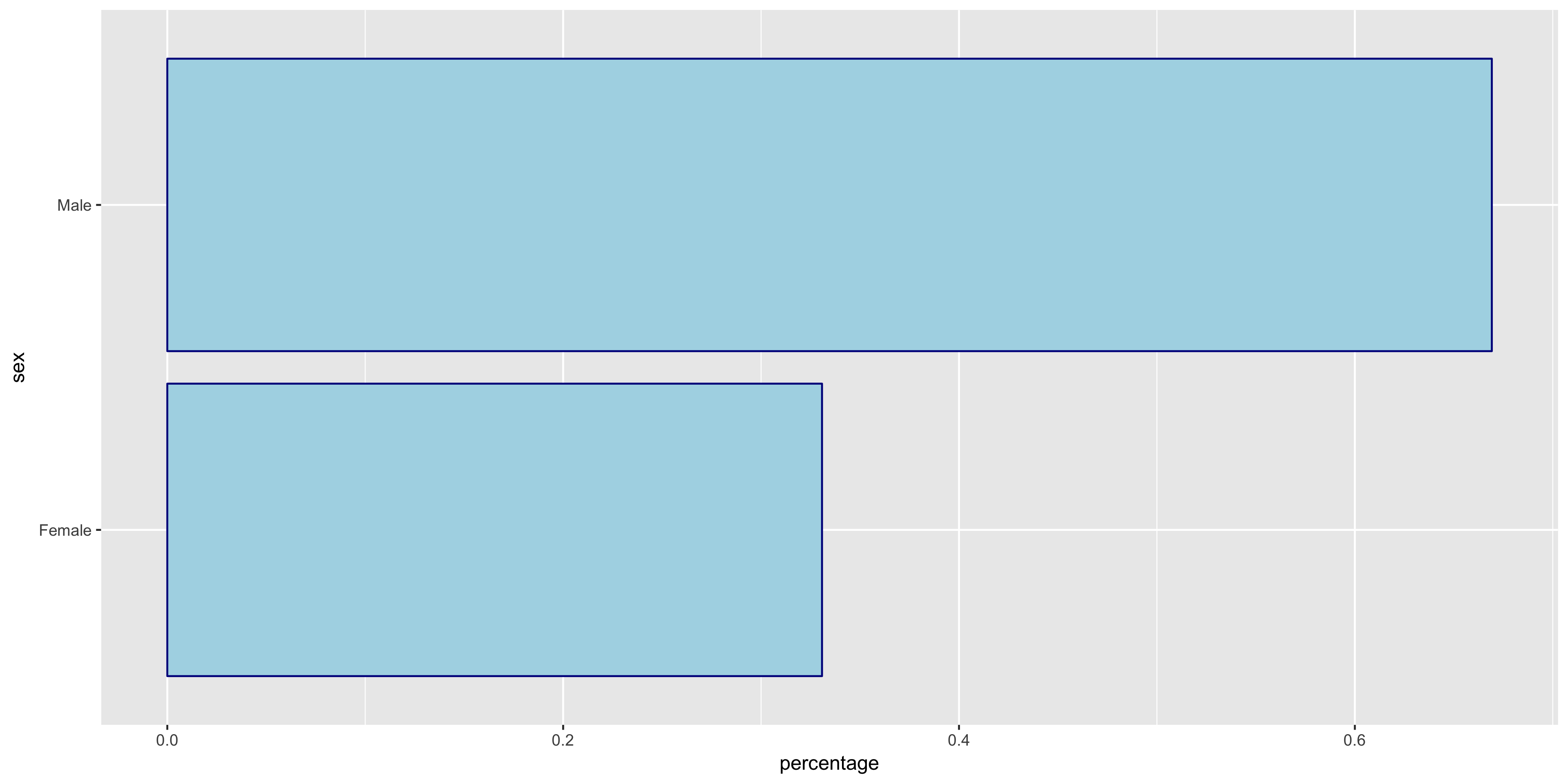
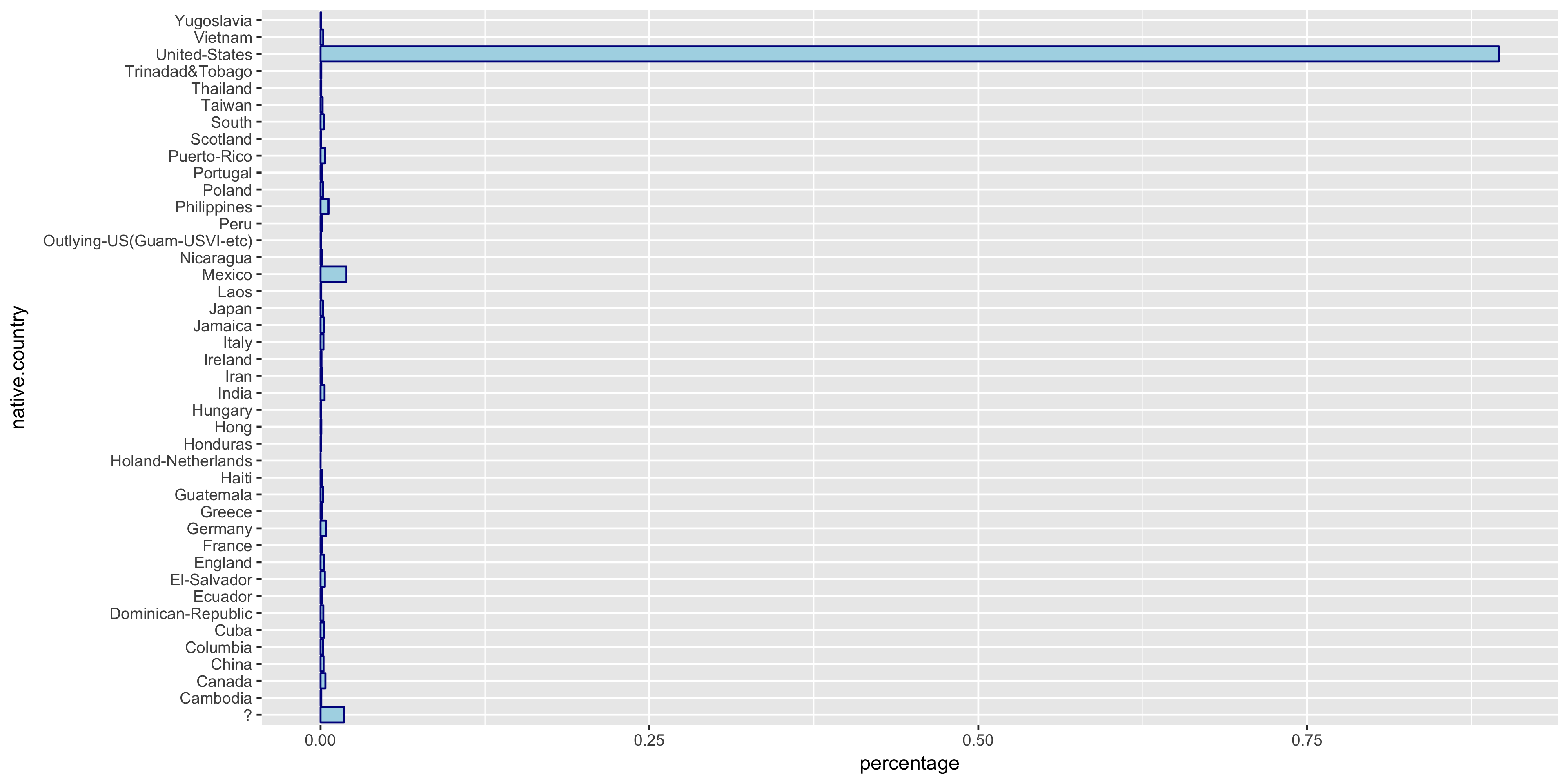
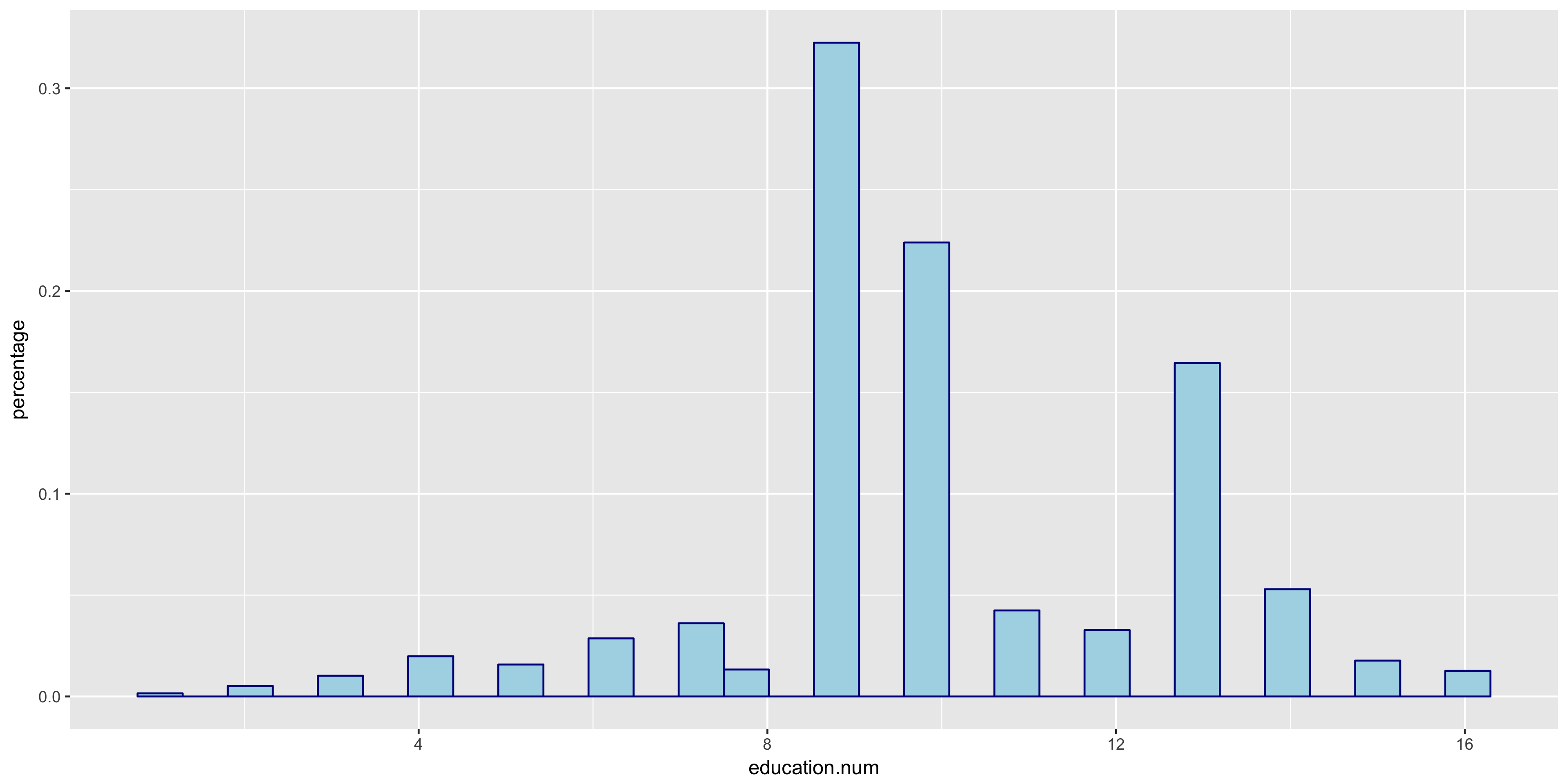
The native.country has a very tight distribution with 89.59% of the population having a native country of the United States. For this reason, I will not include native.country in my model. In addition, the education variable seems to perfectly correlate with the education.num year value - that is, a value of HS-grad in education correlates with 12 years in education.num. Thus since education.num is finer grained, I chose to only include education.num in my model.
To further investigate the discrete variables, I created stacked bar graphs to include the relative frequencies of >50K and ≤50K.
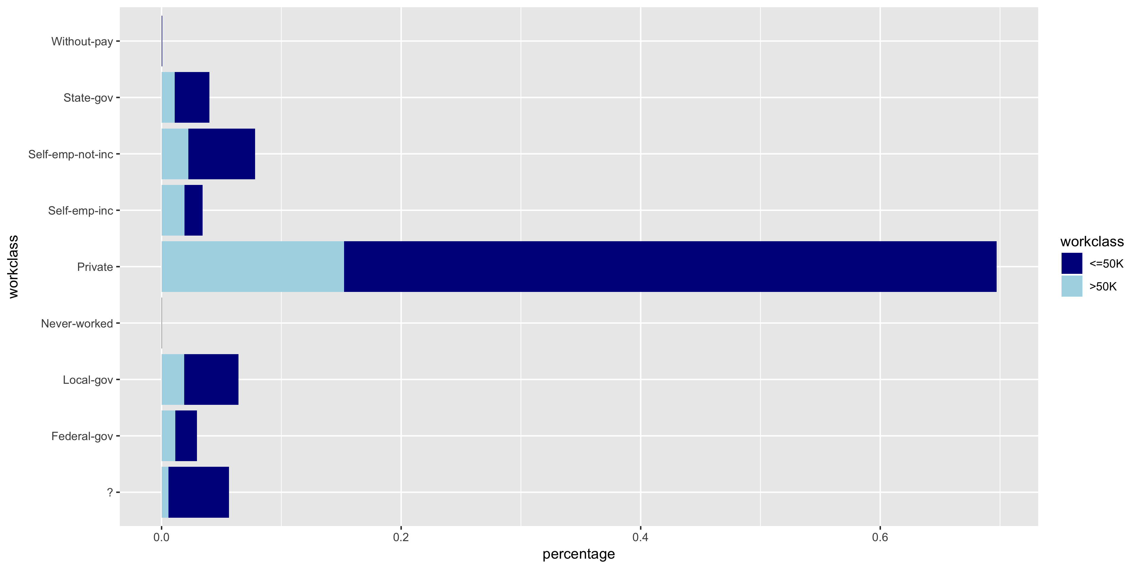
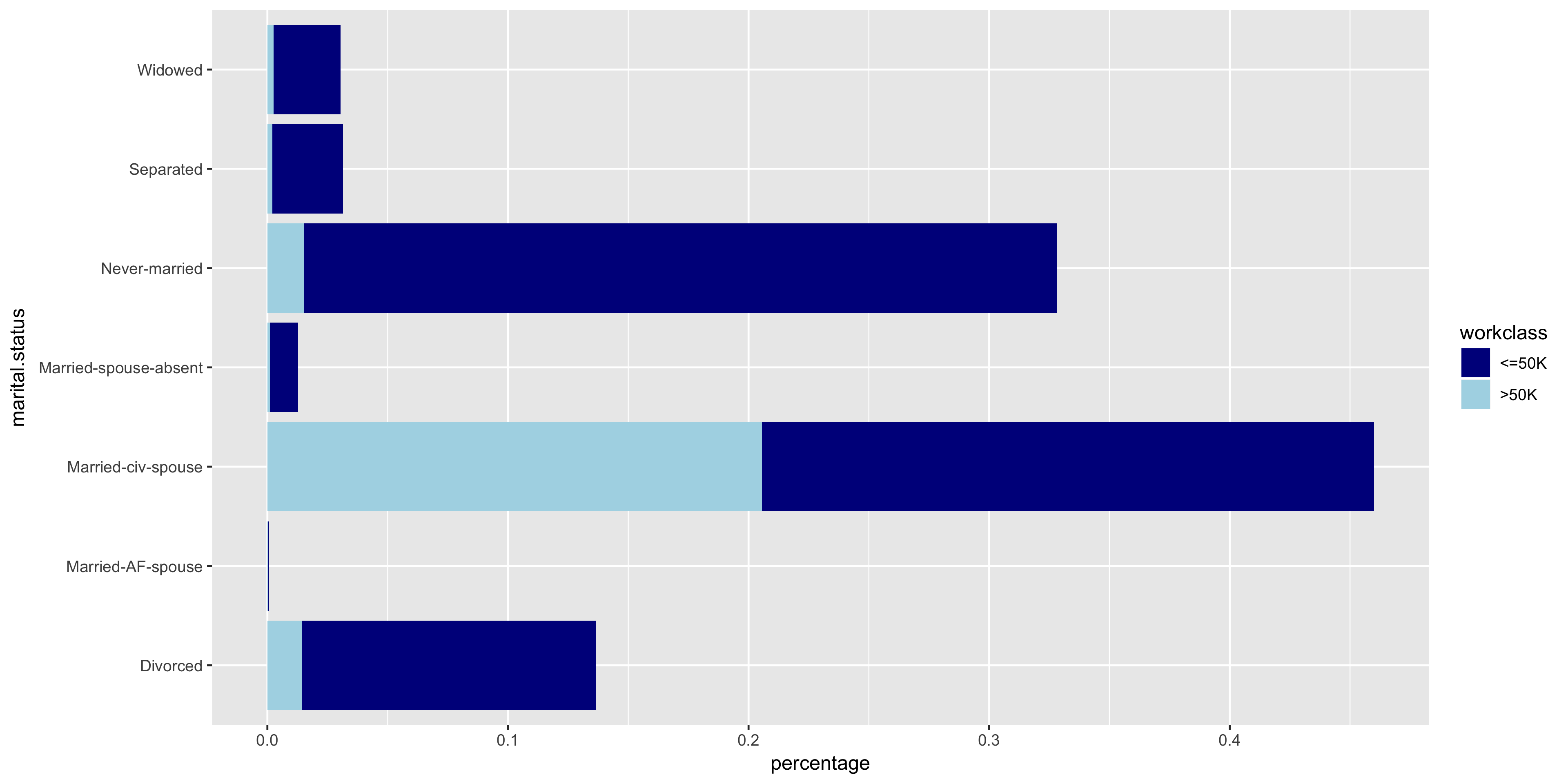
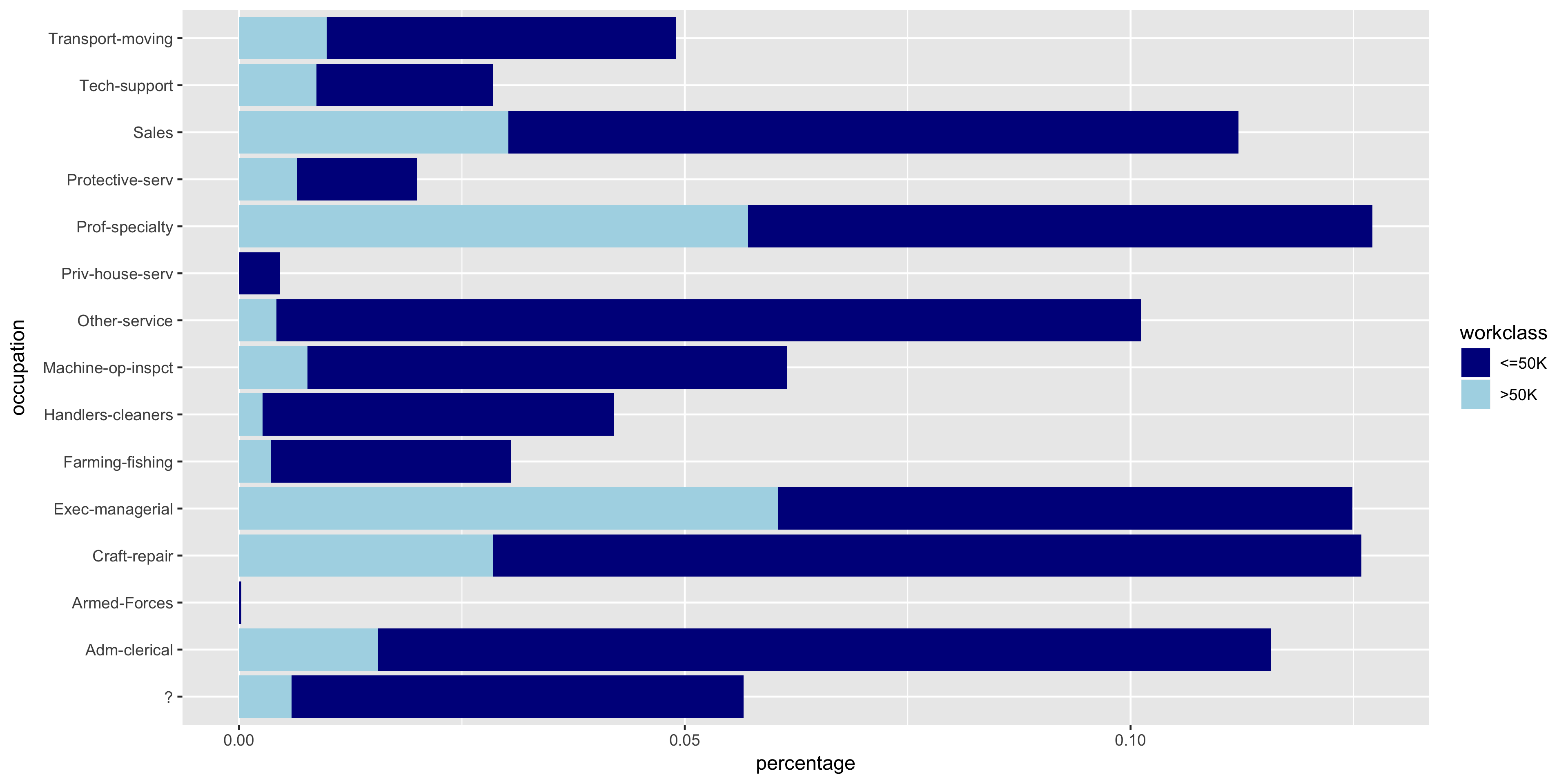
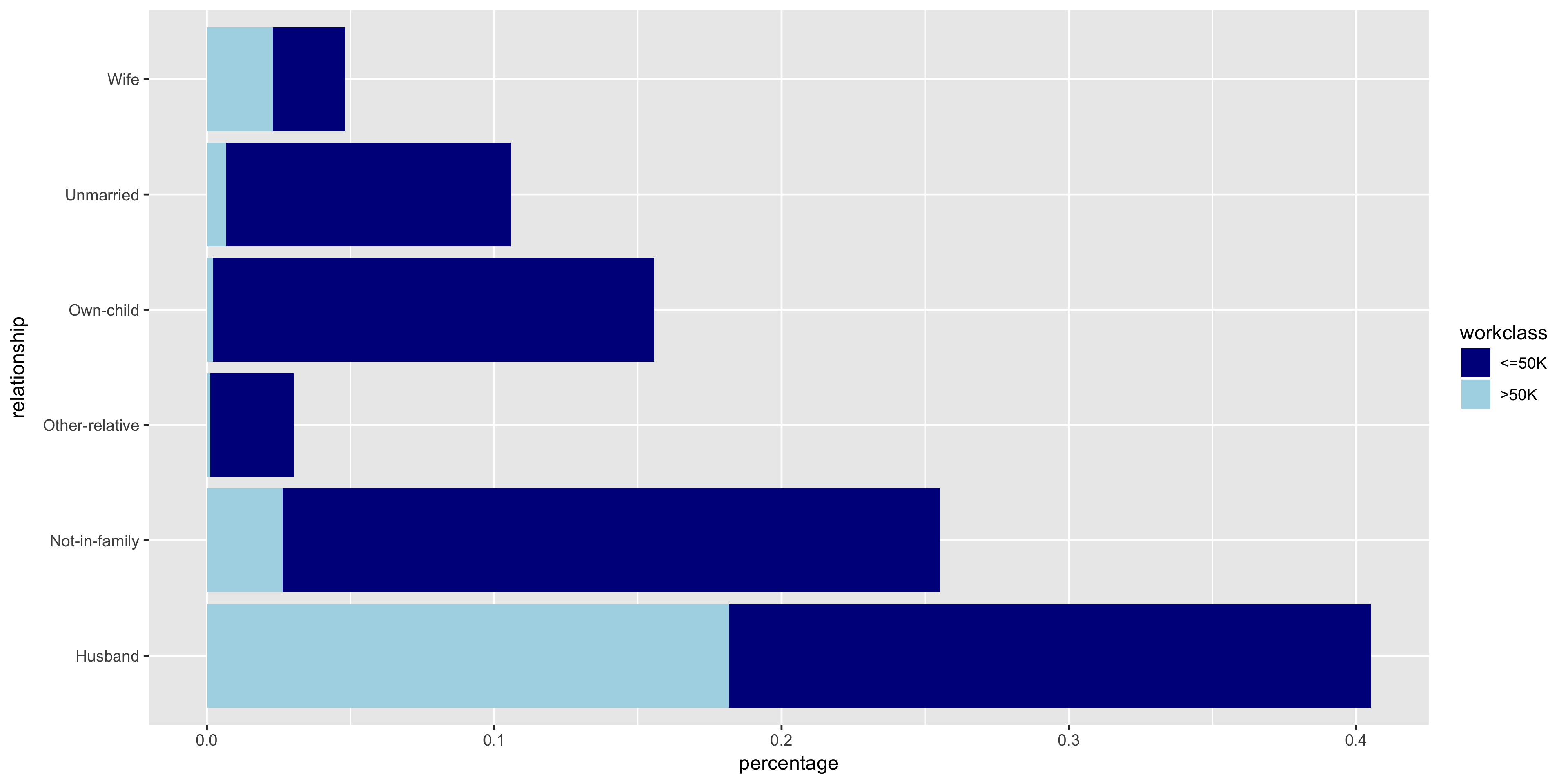
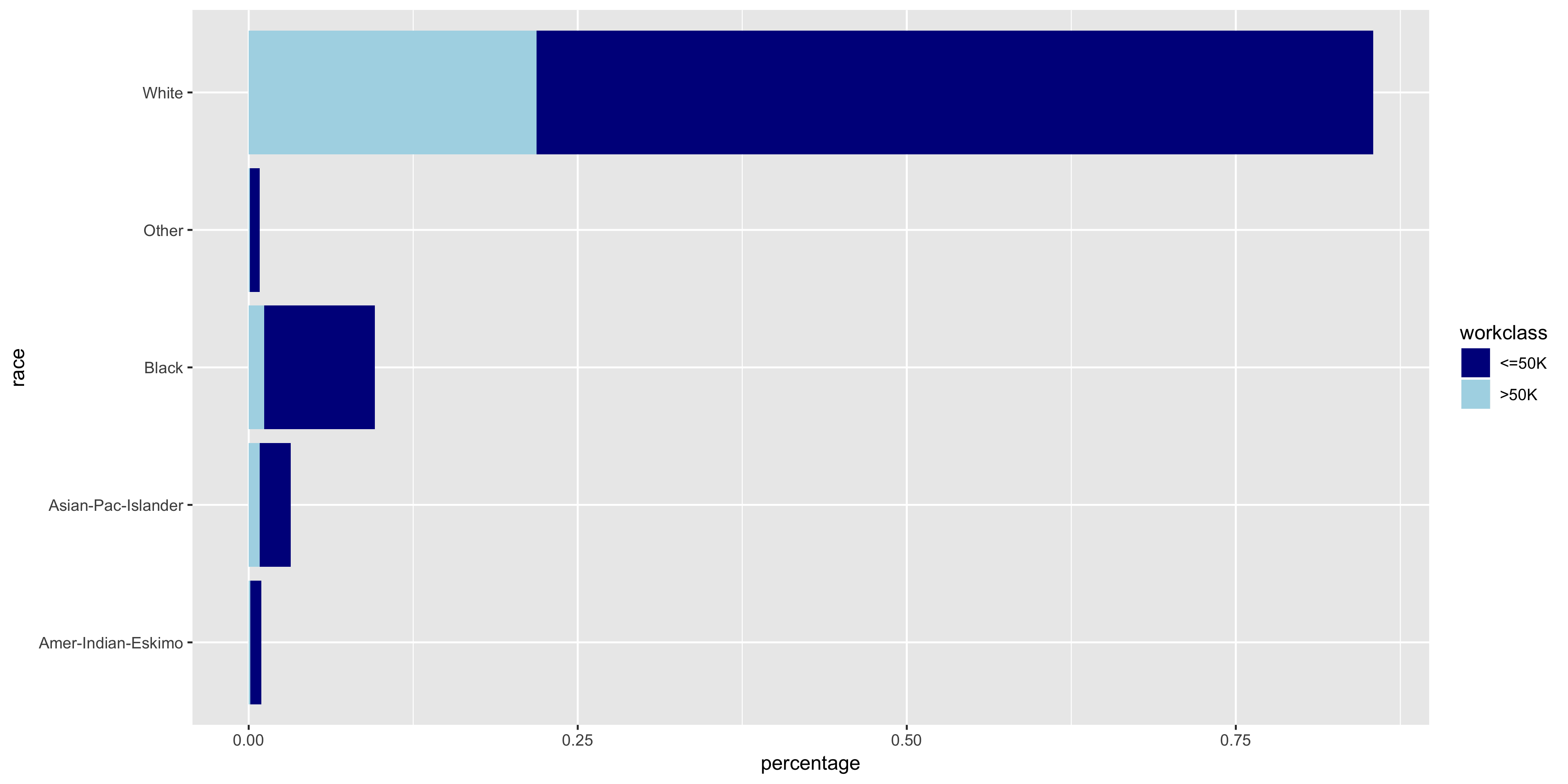
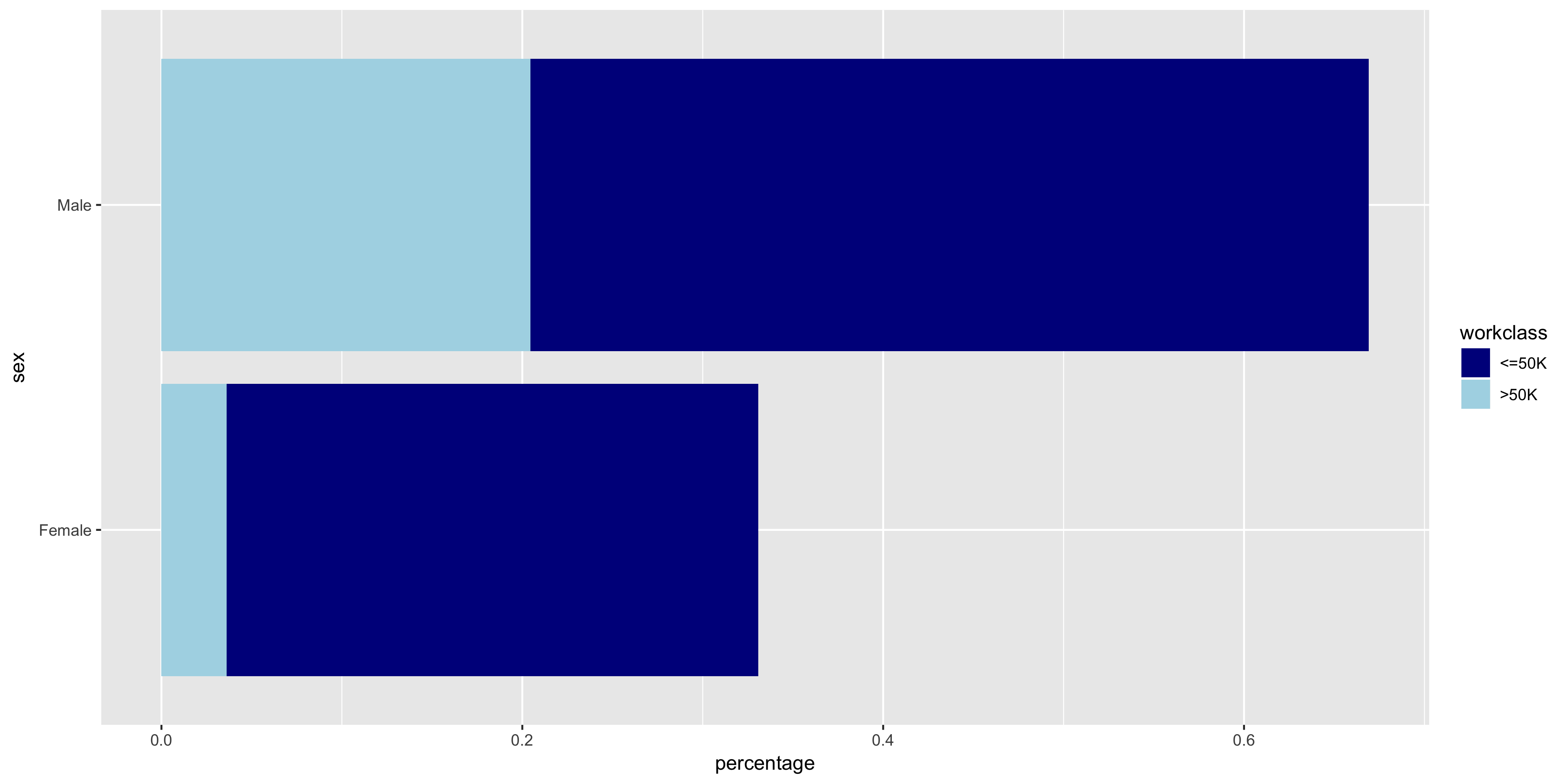
The variables all seem to have varying distributions, so I will include all of these in my model. It also is apparent from these plots that the distribution of >50K is much larger in male citizens
Model Selection
Since the goal is the classification of a dichotomous variable, I will use a logistic regression model. The features that I included in my model are age, education.num, hours.per.week, workclass, marital.status, occupation, relationship, race, and sex.
Training
Using the glm function in R, I trained my model on the training partition of the dataset.
m <- glm(income ~ age + education.num + hours.per.week
     + workclass + marital.status + occupation + relationship
     + race + sex, family=binomial("logit"), data=train)
sum <- summary(m)$coefficients
sort <- order(sum[,4])
sum <- data.frame(sum[sort,])
print(sum)
The coefficients of the features below show the change in the predicted log likelihood of the outcome for a one unit increase in the feature.
| Feature | Estimate | Std. Error | z-value | Pr(>|z|) |
|---|---|---|---|---|
| hours.per.week | 0.031 | 1.53E-03 | 20.0733 | 1.26E-89 |
| education.num | 0.296 | 8.67E-03 | 34.137 | 2.09E-255 |
| age | 0.0296 | 1.54E-03 | 19.280 | 7.91E-83 |
| (Intercept) | -10.147 | 3.78E-01 | -26.848 | 8.94E-159 |
| workclass Self-emp-not-inc | 0.0753 | 1.28E-01 | 0.586 | 5.58E-01 |
| workclass Never-worked | -9.716 | 1.63E+02 | -0.060 | 9.52E-01 |
| workclass Local-gov | 0.334 | 1.32E-01 | 2.531 | 1.14E-02 |
| workclass Self-emp-inc | 0.770 | 1.40E-01 | 5.500 | 3.81E-08 |
| race Black | 0.385 | 2.18E-01 | 1.768 | 7.71E-02 |
| relationship Not-in-family | 0.565 | 2.51E-01 | 2.248 | 2.46E-02 |
| relationship Wife | 1.360 | 9.52E-02 | 14.287 | 2.65E-46 |
| relationship Unmarried | 0.356 | 2.65E-01 | 1.344 | 1.79E-01 |
| race White | 0.504 | 2.08E-01 | 2.425 | 1.53E-02 |
| occupation Prof-specialty | 0.708 | 8.78E-02 | 8.069 | 7.09E-16 |
| occupation Protective-serv | 0.653 | 1.25E-01 | 5.241 | 1.59E-07 |
| relationship Other-relative | -0.351 | 2.31E-01 | -1.521 | 1.28E-01 |
| race Asian-Pac-Islander | 0.339 | 2.28E-01 | 1.491 | 1.36E-01 |
| occupation Farming-fishing | -0.838 | 1.33E-01 | -6.296 | 3.05E-10 |
| marital.status Married-civ-spouse | 2.080 | 2.54E-01 | 8.194 | 2.54E-16 |
| occupation Craft-repair | 0.194 | 8.08E-02 | 2.403 | 1.63E-02 |
| marital.status Separated | -0.125 | 1.50E-01 | -0.837 | 4.02E-01 |
| sex Male | 0.856 | 7.18E-02 | 11.928 | 8.43E-33 |
| workclass Without-pay | -11.439 | 1.18E+02 | -0.097 | 9.23E-01 |
| relationship Own-child | -0.671 | 2.52E-01 | -2.664 | 7.73E-03 |
| occupation Machine-op-inspct | -0.188 | 1.02E-01 | -1.851 | 6.41E-02 |
| occupation Adm-clerical | 0.121 | 9.38E-02 | 1.291 | 1.97E-01 |
| occupation Priv-house-serv | -2.571 | 1.13E+00 | -2.281 | 2.25E-02 |
| race Other | -0.165 | 3.25E-01 | -0.506 | 6.13E-01 |
| workclass State-gov | 0.156 | 1.43E-01 | 1.093 | 2.74E-01 |
| occupation Armed-Forces | -0.710 | 1.26E+00 | -0.563 | 5.74E-01 |
| marital.status Widowed | 0.113 | 1.39E-01 | 0.813 | 4.16E-01 |
| workclass Private | 0.529 | 1.18E-01 | 4.502 | 6.73E-06 |
| workclass Federal-gov | 0.975 | 1.45E-01 | 6.735 | 1.64E-11 |
| occupation Sales | 0.414 | 8.52E-02 | 4.866 | 1.14E-06 |
| marital.status Married-AF-spouse | 2.450 | 5.43E-01 | 4.513 | 6.39E-06 |
| occupation Other-service | -0.802 | 1.19E-01 | -6.755 | 1.43E-11 |
| occupation Handlers-cleaners | -0.583 | 1.40E-01 | -4.177 | 2.95E-05 |
| marital.status Spouse-absent | -0.087 | 2.08E-01 | -0.421 | 6.74E-01 |
| marital.status Never-married | -0.430 | 7.93E-02 | -5.425 | 5.80E-08 |
| occupation Tech-support | 0.728 | 1.14E-01 | 6.406 | 1.49E-10 |
| occupation Exec-managerial | 0.931 | 8.24E-02 | 11.308 | 1.20E-29 |
By analyzing the feature coefficients, it is apparent that a large number of features are not statistically significant (p > .05), and thus do not contribute meaningfully to the model. These features are bolded and italicized in the table above. It appears that the features I selected through my exploratory data analysis are not be the most optimal subset of features. Let’s see if we can do better.
The Lasso Technique
The Lasso is a feature selection and shrinkage method for linear models. The name, Lasso, is actually an acronym for Least Absolute Selection and Shrinkage Operator. The Lasso estimate is defined as:
In this case, the tuning parameter controls the effect of the penalty.
In R, we can use the glmnet function to find the optimal value for lambda.
cv.out <- cv.glmnet(x,y,alpha=1,family="binomial", type.measure = "mse")
This function outputs two values: lambda.1se and lambda.min. lambda.min is the best model with the lowest CV error. lambda.1se is the value of lambda that is a simpler model than lambda.min, but still maintains an error within 1 standard error of the best model. I chose to use lambda.1se versus lambda.min since it is a simpler model with an error that is comparable to the best model. The simpler model is preferable because it is less prone to overfitting.
The resulting feature coefficients and odds ratio are listed below.
| Feature | Coefficients | Odds Ratio |
|---|---|---|
| (Intercept) | -8.115833261 | 0.000298771 |
| age | 0.022234722 | 1.022483756 |
| workclass Federal-gov | 0.42175318 | 1.524632169 |
| workclass Private | 0.032164565 | 1.032687436 |
| workclass Self-emp-inc | 0.194814933 | 1.215086093 |
| workclass Self-emp-not-inc | -0.263976328 | 0.767991719 |
| workclass State-gov | -0.013690425 | 0.986402862 |
| education Assoc-acdm | -0.120690198 | 0.886308498 |
| education Prof-school | 0.070479572 | 1.07302265 |
| education.num | 0.271707016 | 1.31220249 |
| marital.status Married-AF-spouse | 1.476782832 | 4.378835544 |
| marital.status Married-civ-spouse | 1.759282125 | 5.808266286 |
| marital.status Never-married | -0.322028381 | 0.724677623 |
| occupation Exec-managerial | 0.688178679 | 1.990087641 |
| occupation Farming-fishing | -0.778132972 | 0.459262668 |
| occupation Handlers-cleaners | -0.379597994 | 0.684136381 |
| occupation Machine-op-inspct | -0.14071935 | 0.868733088 |
| occupation Other-service | -0.58675557 | 0.556128682 |
| occupation Prof-specialty | 0.409664395 | 1.506312174 |
| occupation Protective-serv | 0.279387174 | 1.322319212 |
| occupation Sales | 0.170704398 | 1.186140072 |
| occupation Tech-support | 0.435470246 | 1.545689743 |
| relationship Other-relative | -0.182299291 | 0.833351889 |
| relationship Own-child | -0.621429641 | 0.537175919 |
| relationship Wife | 0.878403791 | 2.407054476 |
| race White | 0.102088171 | 1.107481115 |
| sex Male | 0.545103832 | 1.724787461 |
| capital.gain | 0.0002304 | 1.000230427 |
| capital.loss | 0.000558734 | 1.00055889 |
| hours.per.week | 0.026468125 | 1.026821517 |
| native.country Cambodia | 0.205780038 | 1.228482954 |
| native.country Columbia | -0.2567686 | 0.773547192 |
| native.country Italy | 0.147862783 | 1.159353802 |
| native.country Mexico | -0.031542921 | 0.968949368 |
| native.country Philippines | 0.031896842 | 1.032410998 |
| native.country South | -0.08434675 | 0.919112498 |
| native.country United-States | 0.099264715 | 1.104358601 |
Model Performance
I used the test partition of the data set as my validation set when performing cross-validation. I predicted the values of the target variable, income, using my new simpler model. Then to test for the model’s accuracy, I constructed a confusion matrix.
lasso.probs <- predict(cv.out, newx=x_test,s=lambda1se, type="response")
lasso.income <- rep(" <=50K.", length(test$income))
lasso.income[lasso.probs >= .5] <- " >50K."
confusion.matrix <- table(test$income, lasso.income)
The resulting confusion matrix is displayed below.
The accuracy of the model when tested against the validation set was 85.21%. The precision of the model was 93.7%.
Conclusion
The largest indicator of a citizen making greater than $50K is having a marital status of ‘married’. The fitted model says that, holding all other variables constant, the odds that a citizen makes over $50K increases by a factor of 4.379 or 5.808 if the citizen is an armed forces married person or a civilian married person, respectively. This may be slightly misleading since households typically complete one census, so the reported income may be a combination of both the spouse’s income. A person is 2.407 times more likely to make over $50K if their relationship status is Wife. This also may be a result of the nature of completing a census as a household.
Another strong indicator is years of education. Controlling for all other variables, for every one year increase in education, the inhabitant is 1.312 times more likely to make more than $50K. Occupations in which one needs higher education, such as executive/managerial, professional/specialty, and tech support positions, also have a positive effect on the odds of making greater than $50K.
In 1994, the gender wage gap appears to have been quite large. The odds that a citizen makes more than $50K increases by a factor of 1.725 if that citizen is male.