Detecting Privacy-Sensitive Objects

The privacy concerns and issues with regard to online social media networks are continually burgeoning as more global users adopt the social platforms. To alleviate these concerns, many social media networks allow users to configure their privacy preferences in a coarse-grained manner. Unfortunately, many users are unaware of the privacy implications that exist with oversharing on social media platforms. Thus, the need arises for an automated approach to analyze photo content and recommend privacy settings to users.

This project is largely inspired by this paper in which the researchers develop a novel approach, iPrivacy, for suggesting privacy settings with deep learning technologies. iPrivacy strives to recommend privacy settings based on the content of the image. I wanted to try to implement a portion of their system as a proof of concept. I was mainly interested in their random walk algorithm which aligns objects with their appropriate privacy labels (more on this later).

About the Data

To train my model to identify private and public objects I have utilized this dataset. The researchers crawled Flickr, and downloaded 90,000 images in 2010. Since labeling such a large scale dataset is difficult and time-consuming, the researchers crowd sourced the picture labeling. They provided the following guidance for users to label the image: “Private are photos which have to do with the private sphere (like self-portraits, family, friends, your home) or contain objects that you would not share with the entire world (like a private email). The rest is public. In case no decision can be made, the picture should be marked as undecidable.”

The creators of the photo dataset provide a cleaned csv file that includes the photo id and the photo’s labeled class. In order to download the actual images, I wrote this simple python script.

import csv #file i/o for original dataset
from requests import get #library used for http web requests
from ast import literal_eval #used to parse response from flickr

#using the flickr api, download the json information for a photo ID
def downloadJSON(photo_id, file_path):
    url = "https://api.flickr.com/services/rest/?method=flickr.photos.getSizes&api_key=cb9885c06e1861ad49bad63b6a6714d9&photo_id=" + photo_id + "&format=json&nojsoncallback=1"
    #get request
    response = get(url)
    #convert byte response to json string format
    json_response = literal_eval(response.content.decode('utf8'))
    if json_response["stat"] == "ok":
        if json_response["sizes"]["candownload"]==1:
            image_url = json_response["sizes"]["size"][-1]['source'].replace("\\", "")
            downloadImage(image_url, file_path)

#using the json output, download the image from the provided link
def downloadImage(url, file_name):
    #open file
    with open(file_name, "wb") as file:
        #get request
        response = get(url)
        #write to file
        file.write(response.content)

dataReader = csv.reader(open('cleaned.csv'), delimiter='\t')

#index 0 represents photoID, index 3 represents private/public class
for row in dataReader:
    if row[3] == "private":
        downloadJSON(row[0], "private/"+row[0]+".jpg")
    if row[3] == "public":
        downloadJSON(row[0], "public/"+row[0]+".jpg")

Once I obtained all of the images that were still available, I had collected 10,427 photos labeled public and 2,275 photos labeled private. This was far fewer than the number of photos I had hoped for, but this was the only publicly available dataset of the sort. The researchers in the iPrivacy paper had a much larger dataset of ~800,000 images which is very helpful when training deep learning models.

Semantic Segmentation

The privacy labels for the dataset are vaguely given at the image level without clear reasoning behind the influences for an image’s privacy labels. Initially, we do not have knowledge of any correspondence between objects in images and the label assigned to the image. To learn the correspondence between objects and privacy settings, we must first have the capability to detect and segment object regions in images. Therefore, the first step of the system, following the collection of the image dataset, is semantic image segmentation.

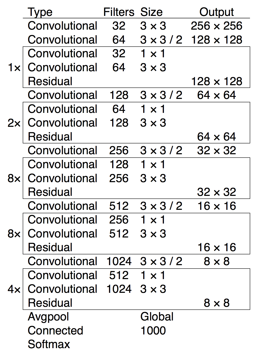
For my project, I leveraged one popular object detector which employs neural networks, YOLO9000. Shortly after I started working on this project, version three of YOLO was released. The upgrade to YOLOv3 included a complete overhaul of the neural network it employs. Version 3 is a hybrid between Convolutional Neural Networks (CNNs) and Residual Neural Networks (RNNs) in that it includes convolutional and residual layers. The new network uses sequential 3x3 and 1x1 convolutional layers; in total it has 53 convolutional layers as seen below.

The architecture of the YOLOv3 neural network.

When presented with a photo, YOLO returns the predicted classes outlined by bounding boxes and their corresponding prediction confidence score. By default, YOLO will return any object that it identifies with a confidence score greater than 0.25.

I wrote a bash script to execute the object detection on each image, and stored the prediction results for object classes and bounding boxes in files which correspond to the original images.

#!/bin/bash
for file in ~/private/*
do
  ./darknet detect cfg/yolov3.cfg yolov3.weights "$file"
  | awk '{if(NR>1)print $1}' | sed 's/\://' >>
  ~/privateResults/"${file##*/}-results.out"
done

I used the weights and configuration for YOLOv3 that were trained against the COCO dataset, indicated by cfg/yolov3.cfg and yolov3.weights. The awk command trims off the first line of output and returns the first column values. The sed command removes the colon from the output, and finally write the results to a new file.

Co-Occurrence Network

After the semantic segmentation process, I constructed a bag-of-words (BoW) model from the resulting files. BoW models are popular feature representation models for text and image classification. In image classification, the BoW model, often referred to as bag-of-visual-words, serves as a vector of occurrence counts for objects in a vocabulary of image features. In this project, the vocabulary of image features is equivalent to the object classes from the COCO dataset. The COCO dataset consists of 80 object classes from the following 9 categories: food, transportation, animals, sports, electronics, furniture, people-oriented, appliances, and miscellaneous. Therefore, for each image, we are projecting its detected object classes over the full set of 80 object classes to obtain an 80-dimensional sparse representation.

Obtaining an Initial Object-Privacy Relevance Score

We use the co-occurrence, $\Psi (C_{i}, t)$, between an object class $C_{i}$ and a given privacy setting $t$ to obtain an initial privacy-relevance score. The privacy settings, i.e. private and public, can be combined to create $P$, a small list of privacy settings. For each privacy setting $t$ , $t \in P$ , its privacy relevance score $\gamma (C_{i}, t)$ with object class $C_{i}$ is given as:

$$\gamma (C_{i}, t) = \Psi (C_{i}, t)$$

It is simple to use co-occurrence because it gives us the probability for an object class $C_{i}$ to be assigned the privacy setting $t$. Co-occurrence is defined as:

$$\Psi (C_{i}, t) = \frac{N(C_{i}, t)}{N(C_{i}, P)}$$

where $N(C_{i}, t)$ is the number of images containing object $C_{i}$ that are labeled $t$, and $N(C_{i}, P)$ is the total number of images containing object $C_{i}$.

Constructing Co-Occurrence Network

For two object classes $C_{i}$ and $C_{j}$, their co-occurrence, $\Psi (C_{i}, C_{j})$, is given as:

$$\Psi (C_{i}, C_{j}) = \frac{N(C_{i}, C_{j})}{N}$$

where $N(C_{i}, C_{j})$ is the number of images containing both object $C_{i}$ and $C_{j}$, and $N$ is the total number of images in our dataset.

We calculated the co-occurrence values for every object class using the aforementioned bag-of-words model, and created a co-occurrence matrix using Python. If you remember some basics of linear algebra, it is simple to calculate the co-occurrence matrix by computing the element-wise dot product of the BoW model with the transpose of the BoW model. In Python, I used the numpy library to perform the calculation. The code snippet is below.

co_occurrence = bag_of_object_classes.T.dot(bag_of_object_classes)
np.fill_diagonal(co_occurrence.values, 0)
co_occurrence.to_csv('co_oc.csv', sep=',')

Note that we assign the diagonal columns to 0 since object classes do not co-occur with themselves.

From the matrix, I created and visualized the network using Gephi. Gephi is popular amongst researchers for visualizing network graphs which includes a large variety of layouts for graphs. In the network, nodes represent objects and the edges between nodes are drawn if $\Psi (C_{i}, C_{j}) > 0$, i.e. if the two objects appear in at least one image together. We also scale the edges to correspond to the value of $\Psi (C_{i}, C_{j})$, i.e. the edges are thicker if the two objects co-occur frequently in images. The layout I used is known as Force Atlas; nodes are assigned a degree-dependent repulsive force and gravity, and the physics simulation aligns the layout of the objects in the network. The object co-occurrence network is illustrated below. The category of the object is represented by the node color.

The co-occurrence network for detected objects.

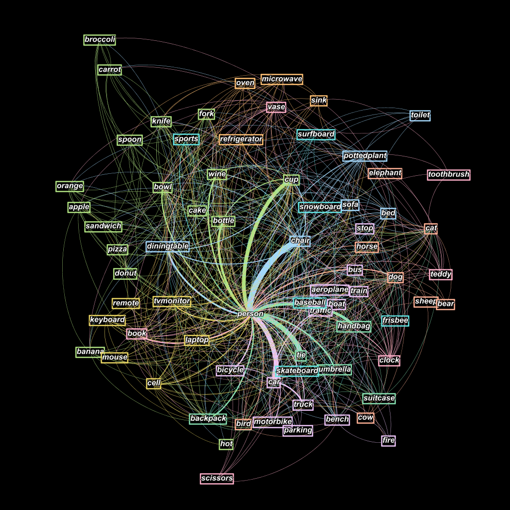
I observed an interesting phenomena in the co-occurrence network. Objects which were manually categorized in the same categories tended to appear near objects in the same category, e.g. objects from the electronics category (remote, keyboard, tv monitor, cell phone) appear in a tight cluster in the bottom left corner.

Object Privacy Alignment

Based on my observations I felt that the network provides a suitable environment for iteratively refining the object-privacy relevance scores. The intuition is that objects which co-exist frequently in images may have similar privacy implications. We follow a random walk process which stochastically traverses the co-occurrence network to more accurately update the object-privacy relevance scores. This was largely based off the referenced paper at the top of the page. We use $p_{k}(C_{i}, t)$ to indicate the object-privacy relevance score between the privacy setting $t$ and the object class $C_{i}$ at the kth iteration. In other words, $\gamma(C_{i} , t) = p_{0}(C_{i}, t)$. We further define a transition probability matrix containing element $\delta_{ij}$ which indicates the transition probability from object $C_{i}$ to its neighbor $C_{j}$. $\delta_{ij}$ is delineated as:

$$\delta_{ij} = \frac{\Psi(C_{i},C_{j})}{\sum_{C_{k}\in\Omega_{C_{i}}}\Psi(C_{i},C_{j})}$$

where $\Omega$ are the neighbors of object class $C_{i}$, and $\Psi(C_{i},C_{j})$ is the co-occurrence value for the object class $C_{i}$ and $C_{j}$ as defined before.

Random Walk

The random walk algorithm that automatically refines privacy-relevance scores is devised as:

$$p_{k}(C_{i}, t) = \theta\sum_{C_{j}\in\Omega_{C_{i}}}p_{k-1}(C_{j}, t)\delta_{ij}+(1-\theta)\gamma(C_{i}, t)$$

where $\theta$ is a weight parameter, $\gamma(C_{i}, t)$ is an object class’s initial privacy-relevance score, and $p_{k-1}(C_{j}, t)$ is the privacy-relevance score for the previous iteration. The weight parameter can be adjusted to increase or decrease the importance of the initial privacy-relevance scores. We empirically found good results using $\theta$ = 0.4. After the random walk process converges, we re-ranked the privacy settings according to the newly updated privacy-relevance scores. An object is classified as the privacy setting with the largest privacy-relevance score.

Constructing Object Privacy Co-Occurrence Network

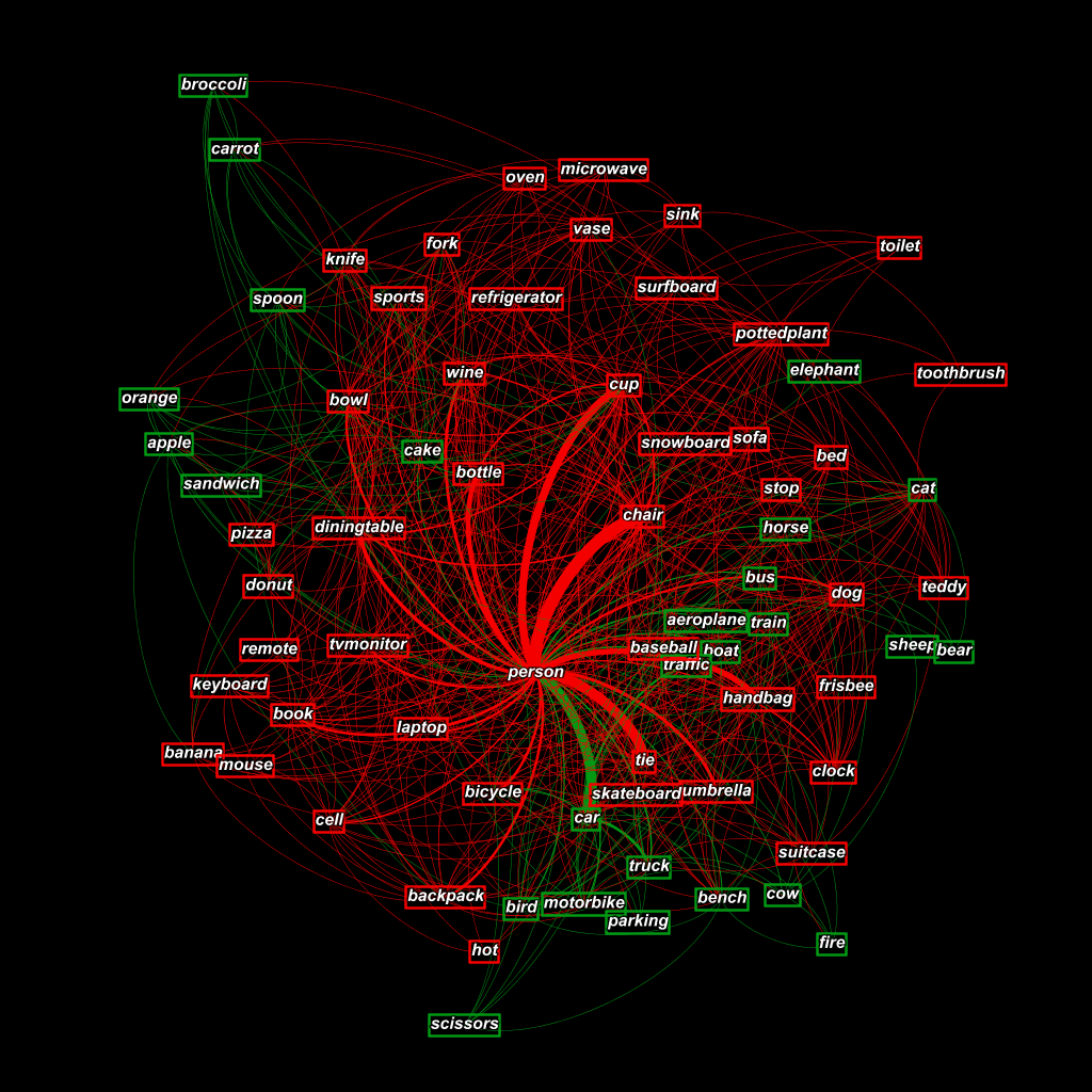
After the successful completion of my analysis, I found 51 private objects and 29 public objects. I visualized the results of the object privacy settings by using the same co-occurrence network. Instead of the initial category colors, I assigned green to public objects and red to private objects. The visualization is illustrated

Red objects represent private objects. Green objects represent public objects.

Discussion

The researchers who created the original dataset provided the following guidance for participants to label images: “Private are photos which have to do with the private sphere (like self-portraits, family, friends, your home) or contain objects that you would not share with the entire world (like a private email). The rest is public.” It appears that the results of my system correspond to the guidance provided by those researchers in that the public objects are those which mainly do not have to do anything with the private sphere of self-portraits, your home, family, or friends. They are objects which appear in photos that are overwhelmingly labeled public, e.g. airplane, bus, train.

The random walk process tends to favor labeling objects as private due to the overwhelming private privacy-relevance score of the person object. However, I feel that it is favorable to be more biased towards private privacy setting than public privacy setting. In a system that is supposed to be protecting users privacy, it would be better to have more false positive errors for private objects. The system would still guarantee privacy leakage is contained, but the downside is that a majority of images would be labeled private.

Another issue with my project was the size of the dataset that I used. Deep learning technologies are notorious for needing large datasets to achieve performance comparable to other machine learning techniques. My dataset was only 12,702 images while the dataset in the original paper was over 800,000 images. The sheer size of data allows for more thorough analyses that I was unable to perform. For example, the author’s cluster images in their dataset which contain similar objects. They further used these clusters to learn the initial privacy-relevance scores. I used K-means clustering to cluster the dataset, and received clusters which were semantically very similar. However, I found that segmenting our already small dataset lead to poor results for the random walk process. As an alternative, for the random walk process, I treated our entire dataset as a singular cluster.

In addition, I feel that we could improve our project results by training YOLO9000 to detect more objects than the 80 object classes provided by the COCO dataset. A large majority of the objects detected by my system do not have a direct influence on the privacy setting of the image. I could train the CNN to detect objects that are socially regarded as private, such as photo IDs, credit cards, license plates, intimate photos, etc.. The addition of such objects could influence the co-occurrence network in a manner that would better align objects with their privacy setting.